In this study, we concluded the prediction methods for identifying m5C modification sites on the same dataset and the current advancements in m5C modification site prediction. Although the Deepm5C model [32] has made quite a lot of progress, there are still some deficiencies to overcome. Therefore, we designed a novel deep-learning model called im5C-DSCGA to identify m5C modification sites in human RNA.

Fig. 1 summarizes the design of the prediction and evaluation processes for the im5C-DSCGA model. This process consisted of four parts, respectively: feature encoding, im5C-DSCGA model framework, ensemble learning module, and performance evaluation. In the feature encoding part, we used three encoding methods, namely, one-hot encoding, nucleotide chemical property (NCP), and nucleotide density (ND). In the model framework part, for a given RNA sequence, the network framework consists of six modules, which are the input module, improved DenseNet module, improved CBAM Attention module, BGRU module, Self-Attention module, and output module. The input module is used to feed the original RNA sequences into the subsequent DenseNet module after three kinds of features are encoded. Then, using the improved DenseNet module, the network can extract more advanced features than the residual networks and ordinary convolutional neural networks. The improved CBAM Attention module is used to extract more critical and prominent features by multiplying the Spatial Attention module and the Channel Attention module at the corresponding positions of their respective feature matrices. The BGRU module also used the output feature vector above as an input. The BGRU module is designed to obtain long-term dependencies between high-level features more efficiently than gated recurrent unit (GRU) and ordinary recurrent neural networks. The Self-Attention mechanism module is used to evaluate the importance of RNA sequence features. The output module uses a fully connected neural network to receive these high-level features as the input and calculates probability values between 0 and 1 using the softmax activation function. In the Ensemble learning model section, we used the homogeneous ensemble [34] method, which ultimately uses soft voting for classification. Here, the average of the three probability values was taken to obtain the final prediction probability. If the probability value is greater than 0.5, a m5C modification site is identified; conversely, the opposite is true. In the performance evaluation section, we show the evaluation of the im5C-DSCGA model by cross-validation and independent tests.

Fig. 1.

The im5C-DSCGA model structure. (A) Feature encoding. RNA sequences were feature encoded using one-hot, NCP, and nucleotide density (ND) to obtain an 8 $\times$ 41 feature matrix. (B) im5C-DSCGA model framework. The final predictor is called “im5C-DSCGA”, where “i” stands for “identification”, “m5C” stands for “m5C modification sites”, “D” stands for using the improved Densely Connected Convolutional Networks (DenseNet), “SC” stands for using the improved Convolutional Block Attention Module (CBAM), “G” stands for using bidirectional gated recurrent unit (BGRU), and “A” stands for using the Self-Attention mechanism. The feature matrix was fed into the DenseNet module after three encodings and the improved CBAM Attention module was subsequently introduced to extract more critical features. A fully connected neural network was used to output the predicted probabilities. (C) Ensemble learning module. The model was verified using five-fold cross-validation, where each fold was tested using an independent test set. Five prediction probabilities are generated for each test RNA sequence and a soft vote was used to determine the final classification. (D) Performance evaluation. We show the evaluation from cross-validation and independent tests. GRU, gated recurrent unit.

The ResNet [23] is an improved convolutional neural network that solves the degradation problem, which can occur in the CNNs, as shown in Fig. 2. It is shown that the overall performance of the CNN is largely affected by the number of network layers. Specifically, the more layers the neural network has, the more complex feature extractions the network can perform, and theoretically improved results can be achieved. Nevertheless, the accuracy saturates or even decreases when the depth reaches a certain level. This is known as the degradation problem and makes it increasingly difficult to train deeper neural networks. However, the residual network uses shortcut connections to solve the problem of model degradation in deep networks. The shortcut connections are added between the other two layers compared to the traditional neural networks, and the deeper layers are brought into play by residual learning. As the number of network layers increases, the residual convolutional neural network can obtain better learning results.

Fig. 2.

The residual neural network (ResNet) structure.

The residual neural network is composed of a series of basic blocks called residual blocks and learns the required mappings and uses a special short-circuiting mechanism to connect them. The residual is the difference between the observed value and the estimated value. Suppose within a certain layer that the solved mapping (optimal function) is noted as $H(x)$, i.e., the observed value, while the feature mapping of the output of the previous residual block is $x$, i.e., the estimated value, then, the residual mapping function $F(x)$ (the fitted objective function) of the network is defined as:

(1)$$F(x)=H(x)-x$$

where the function $F\left(x\right)$ is called the residual function. The existence of the optimal function avoids the problem of negative optimization, while the residual function can better learn the features of the deep network. The shortcut connections of the ResNet are shown in Fig. 3.

Fig. 3.

The ResNet shortcut connection.

Residual Block

A ResNet is composed of a series of basic blocks called residual blocks. For the residual block, we used a three-layer bottleneck structure, which can be seen in Fig. 4. It reduces the size of the feature map by 1 $\times$ 1 convolutional kernels, meaning that the number of 3 $\times$ 3 convolutional kernels is not affected by the input of the previous layer, and its output does not affect the next layer. The middle 3 $\times$ 3 convolutional layer is first down-dimensioned under a 1 $\times$ 1 convolutional layer and then up-dimensioned under another 1 $\times$ 1 convolutional layer. This maintains the model accuracy and reduces the network parameters and computation, thus, saving computation time.

Fig. 4.

The residual block structure.

Traditional CNNs may suffer from inadequate feature extraction, which can lead to network degradation. DenseNet are an improved convolutional neural network that is based on the ResNet. A convolutional layer, the dense block layer, and the transition layer form its network architecture. The RNA sequences are encoded by three feature encoding methods and the feature matrix is first passed through a convolutional layer, then, the dense block layer, and finally the transition layer. In this study, we improved the original network structure of DenseNet. In detail, we removed one layer of the convolutional layer and the feature matrix that RNA sequences were encoded by and three feature encoding methods were directly input into the dense block layer, and a batch normalization layer was added between the dense block layer and the transition layer to, finally, obtain the high-level features of the RNA sequences.

The improved DenseNet extracts the original feature information for RNA sequences at a deeper level and enhances the robustness of the im5C-DSCGA model, resulting in better generalization ability. Fig. 5 shows the network structure of the improved DenseNet.

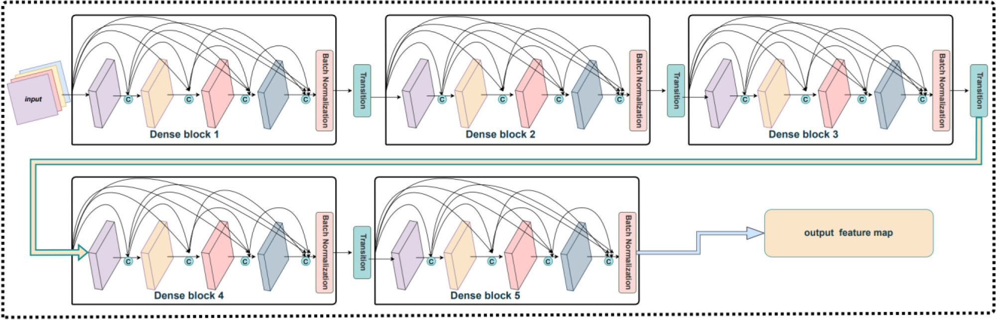Fig. 5.

The improved DenseNet structure.

2.2.3.1 Dense block

The DenseNet uses a dense block structure, which is a dense connection mechanism. It is used specifically to concatenate the outputs of all the previous convolutional layers together as the input of the next convolutional layer, to achieve feature reuse. The dense block structure improves the efficiency of the model and also enhances its expressiveness.

Fig. 6 presents the network structure of the dense block, which consists of the L-layer network structure with a nonlinear transformation function. The nonlinear transformation function consists of a 3 $\times$ 3 convolution kernel and a batch normalization (BN). The Lth layer of the DenseNet receives all the feature map outputs from the previous L-1 layers. The computational formula for its output is expressed as:

(2)$$x_L=H_L\left([x_0,x_1,\mathrm{\dots },x_{L-1}]\right)$$

where $L$ denotes the number of layers, $x_L$ denotes the output of $L$layers, and $H_L$ denotes a nonlinear transformation. $[x_0,x_1,\mathrm{\dots },x_{L-1}]$ denotes the feature map that connects layer 0th to layer L-1th.

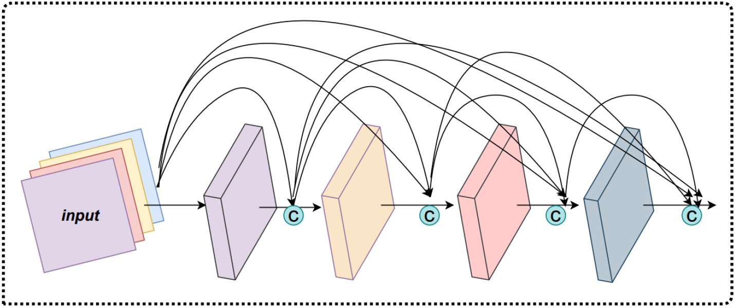Fig. 6.

The dense block structure.

Since considering the various importance of the different features, we introduced an improved CBAM Attention [25] module after the DenseNet module to weight the feature mapping, thereby allowing the further improvement of the prediction ability by the im5C-DSCGA model. The CBAM Attention is a simple and effective attention mechanism in feedforward convolutional neural networks, which includes two modules, a Channel Attention module, and a Spatial Attention module, as shown in Fig. 7.

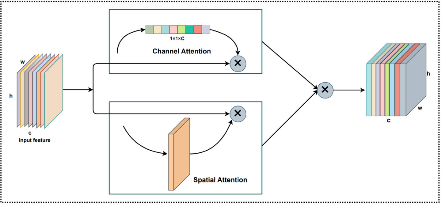Fig. 7.

The improved CBAM Attention module structure.

The original CBAM Attention first evaluates the original features using the Channel Attention module, after which it feeds the feature map produced by the Channel Attention module back to the Spatial Attention module, which then outputs the feature map. However, this serial connection has the drawback of calculating in a particular way, which might result in improper weight calculation in the Spatial Attention module and loss of channel weight information in the finished feature map. Therefore, we improved the CBAM Attention with the idea that the output features from the DenseNet module are fed into the Channel Attention and Spatial Attention modules, multiplying the feature maps of these two outputs by each other at the corresponding positions. By using this approach, we can increase the expressiveness of the features and maximize their retention for each attention module after evaluation.

2.2.4.1 Channel Attention

Considering that the channels in the feature map are different, it has varying degrees of importance. Therefore, we used Channel Attention to compute various weights for each channel, and the structure is shown in Fig. 8. Channel Attention compresses the feature map in the spatial dimension to obtain a one-dimensional vector before manipulating it.

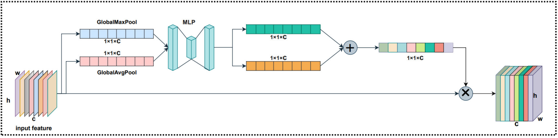Fig. 8.

The Channel Attention structure.

When compressing in the spatial dimension, the Spatial Attention considers both the global average pooling and the global max pooling. For Channel Attention, global max pooling is used to extract the maximum value of the feature map for each channel, while global average pooling is used to extract the average value of the feature map for each channel. Channel Attention is first aggregated by two parallel average pooling and max pooling to aggregate the spatial information of the feature mapping and sent to a shared fully connected neural network (MLP). Secondly, the weights of the Channel Attention module are obtained using the sigmoid activation function after the two results output by the MLP are added element by element. Finally, to obtain the feature map of the Channel Attention module weights, these weights are multiplied by the input feature map. It is possible to express the Channel Attention as:

(5)$${\mathrm{M}}_{\mathrm{c}}(\mathrm{F})=\sigma (\mathrm{MLP}(\mathrm{AvgPool}(\mathrm{F}))+\mathrm{MLP}(\mathrm{MaxPool}(\mathrm{F})))$$

(6)$$Y=F_{\text{scale}}(F,M_c(F))=M_c(F)\cdot F$$

where pooling is global max pooling and global average pooling, $\sigma$ represents the sigmoid activation function. $Y$ represents the final output feature matrix, $M_c\left(F\right)$ represents the weight vector, and $F$ represents the input channel matrix.

2.2.4.2 Spatial Attention

Considering that the receptive domains are different, the degree of their influence on the feature map is also different. Therefore, to calculate the weights between the receptive domains, we employed Spatial Attention. The structure for Spatial Attention is illustrated in Fig. 9. Spatial Attention is compressed for channels, and global max pooling and global average pooling are performed in the channel dimension, respectively. For Spatial Attention, the operation of global max pooling is to extract the maximum value at each position on the channel, while the operation of global average pooling is to extract the average value at each position on the channel. Spatial Attention is firstly processed by two parallel global max pooling and global average pooling operations for feature mapping, and the two obtained feature maps are performed in CONCAT based on the channels. Secondly, after a convolution operation, it can be down-dimensioned to 1 channel before the Spatial Attention feature map is generated by the sigmoid function. The final generated features are obtained by multiplying this feature map by the Spatial Attention input feature map. The Spatial Attention can be expressed as:

(7)$$M_s(F)=\sigma \left(f^{7\times 7}([\mathrm{AvgPool}(F);\mathrm{MaxPool}(F)])\right)$$

(8)$$Y=F_{\text{scale}}(F,M_s(F))=M_s(F)\cdot F$$

where pooling is global max pooling and global average pooling and $\sigma$ represents the sigmoid activation function. The size of the convolution kernel used in the convolution operation is 7 $\times$ 7. $Y$ represents the final output feature matrix, $M_c\left(F\right)$ represents the weight vector, and $F$ represents the input channel matrix.

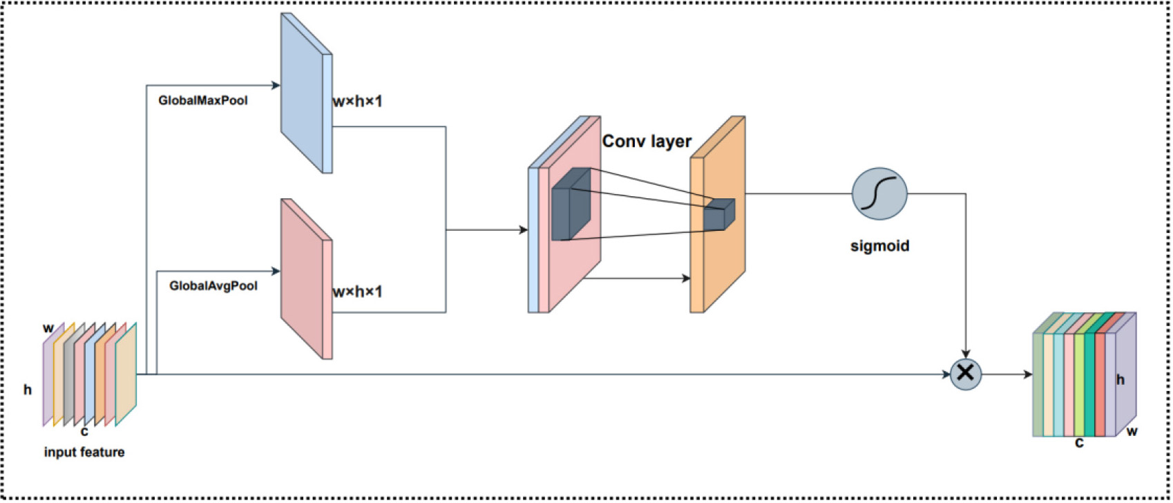Fig. 9.

The Spatial Attention structure.

The bidirectional gated recurrent unit (BGRU) [28] is a recurrent neural network (RNN), which is a variant of the traditional RNN. It is capable of learning long-term dependencies between sequences in RNA sequence prediction tasks and mitigating gradient disappearance or explosion phenomena. Fig. 10 illustrates the BGRU network structure. The BGRU consists of a forward GRU and a reverse GRU. The network of the GRU is simpler compared to the long short-term memory network (LSTM) [35], which synthesizes the forgetting gate and the input gate into a new gate called the update gate. The update gate controls the amount of data that previous memory information continues to be retained until the current moment. Although there is one less gate, there are fewer parameters and GRU can save a lot of time in case of a large training dataset. For a GRU, it can be expressed as:

(9)$$\begin{array}{c}\hfill r_t=\sigma \left(W_{t}x+U_t{h}_{t-1}\right)\hfill \\ \hfill z_t=\sigma \left(W_z{x}_t+U_z{h}_{t-1}\right)\hfill \\ \hfill \widetilde{h_t}=\mathrm{tanh }\left(W{x}_t+U\left(r_t\odot h_{t-1}\right)\right)\hfill \\ \hfill h_t=\left(1-Z_t\right)\odot h_{t-1}+Z_t\odot \widetilde{h_t}\hfill \end{array}$$

where $z_t$ denotes the update gate, $r_t$ denotes the reset gate, $h_t$ denotes the hidden state at the current moment, and $h_{t-1}$ denotes the hidden state at the previous moment. $\odot$ denotes the element multiplication, $\sigma$ is the sigmoid activation function, and W and U are the weight matrices.

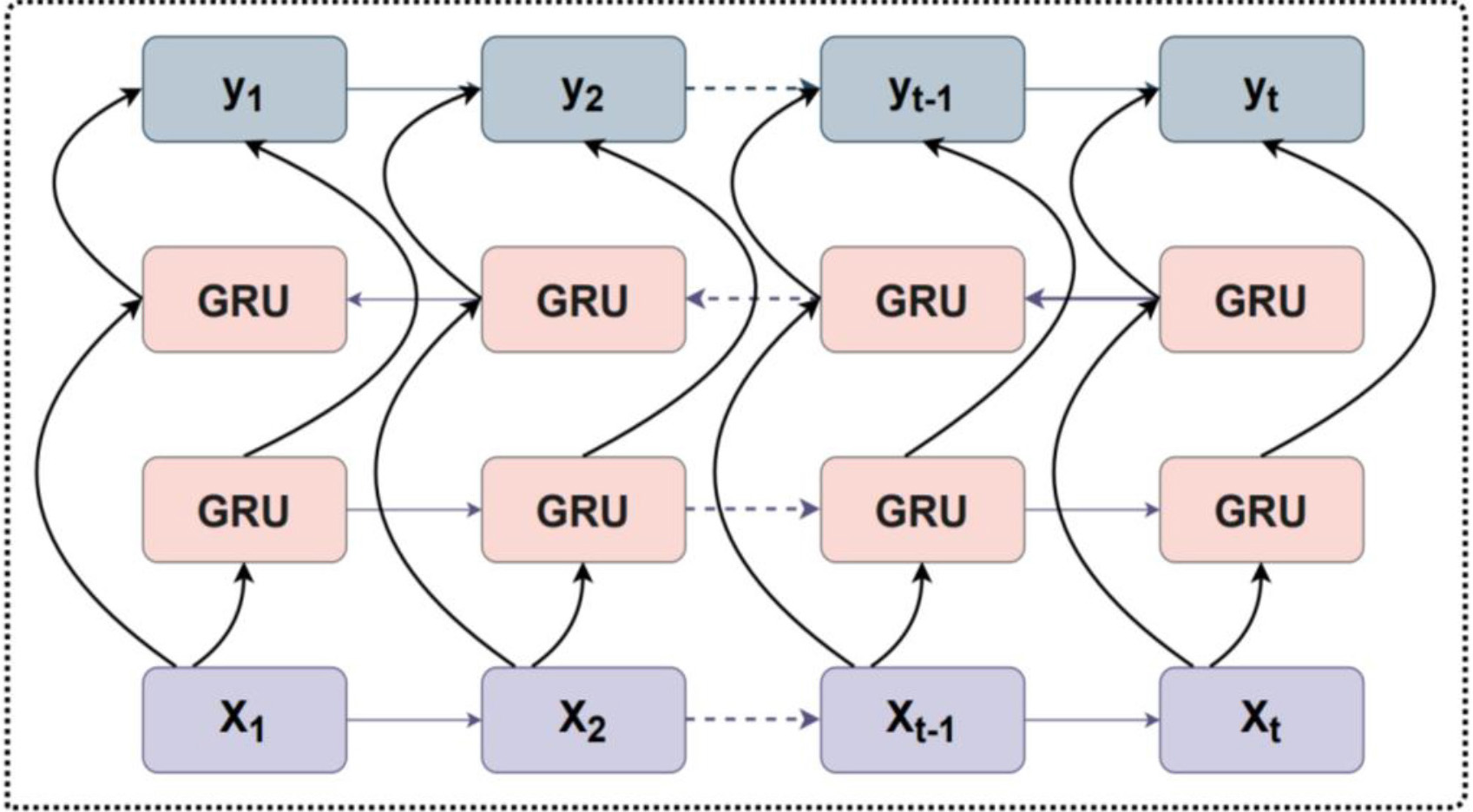Fig. 10.

The bidirectional gated recurrent unit (BGRU) structure.

The Self-Attention [30] mechanism is a widely used mechanism in deep learning, and the specific structure is shown in Fig. 11. It is actually a weighting method, whereby a certain part of the input sequence is given a higher weight than other parts. It can be understood since it wants the machine to notice the correlation between the different parts in the whole input features so that it can better capture the information in the input features.

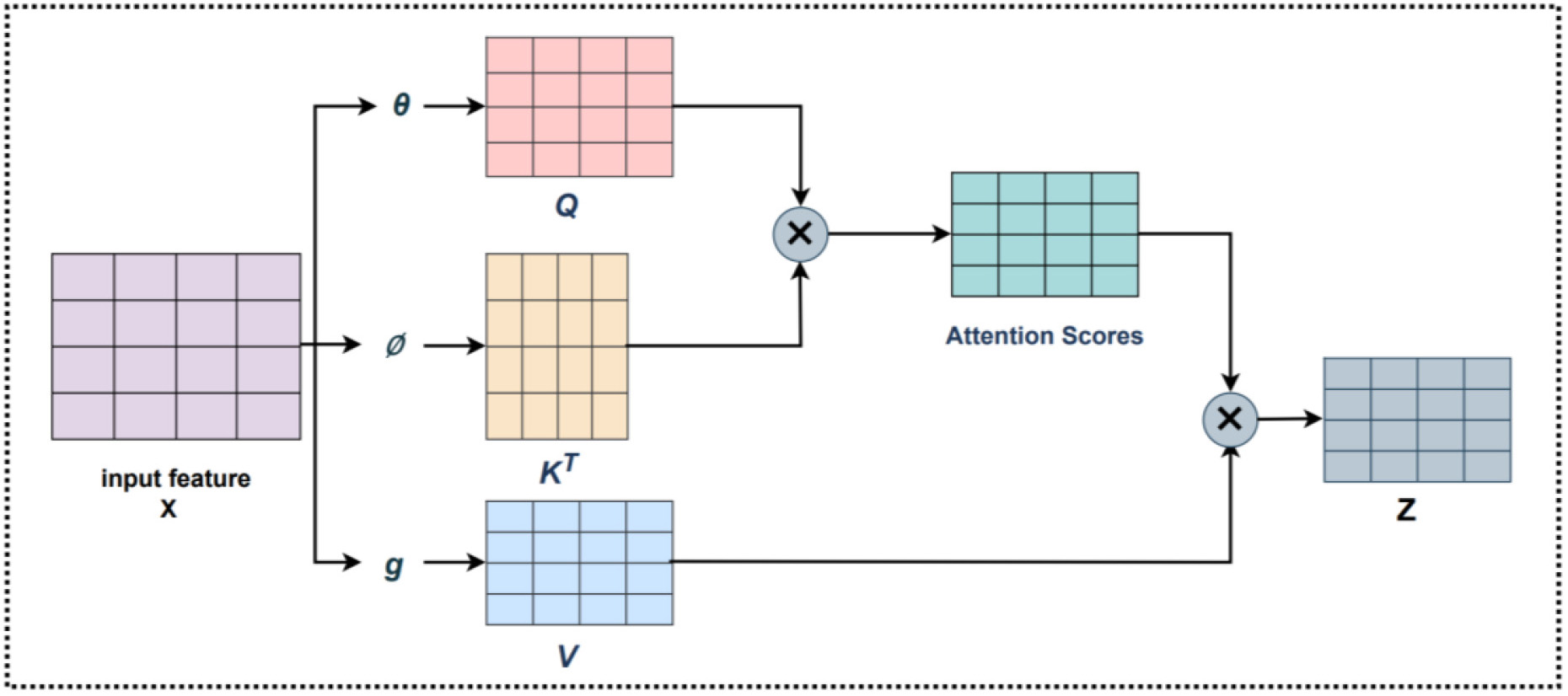Fig. 11.

The Self-Attention structure.

The Self-Attention mechanism converts the input data into three vectors $q_i$, $k_i$, and $v_i$, with query Q as the giver, key K as the receiver creating the relationship, and value V extracting the information and summarizing all relationships in order. Then, each input base is compared to all other bases in the input sequence to determine a score. The score is calculated by multiplying the query vector $q_i$ by the key vector $k_i$, and dividing it by the square root of the key vector dimension. To obtain a probability value from 0 to 1, the score is passed through a softmax operation and multiplied by each value vector. Finally, the value vector $v_i$, at the current input, is weighted and summed to calculate the output vector. Fig. 12 illustrates the process of the Self-Attention mechanism calculation. The weighted value $V$ output vector $O_s$ is represented as:

(10)$$O_s=\phi \left(\frac{Q{K}^T}{\sqrt{d_k}}\right)V$$

where $\phi$ is the softmax function and$d_k$ is the dimension of K.

It is obtained by querying the correlation of the vector with the corresponding vector to calculate the weight of each value vector. The calculation method is shown as:

(11)$$\begin{array}{c}\hfill q_i=W_q{b}_i\hfill \\ \hfill k_i=W_k{b}_i\hfill \\ \hfill v_i=W_v{b}_i\hfill \\ \hfill w_{ti}=\frac{\mathrm{exp }\left(\mathrm{similarity }(h_i,h_j)\right)}{{\sum }_{i=1}^t\mathrm{exp }\left(\mathrm{similarity }(h_i,h_j)\right)}\hfill \end{array}$$

where $W_q$, $W_k$, and $W_v$ are the parameter matrices; $q_i$, $k_i$, and $v_i$ stand for the query, key, and value vectors, respectively; $w_{ti}$ is the weight assignment to the input vectors.

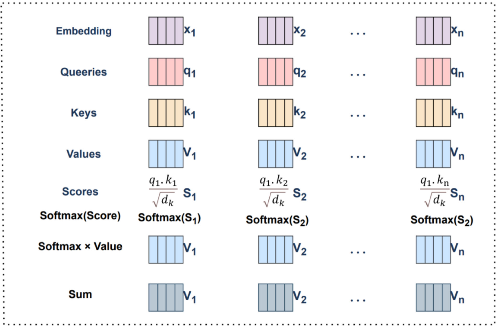Fig. 12.

Self-Attention mechanism calculation using vectors.

In machine learning, the independent test datasets are taken and fed into several identical or different models, to compute several predictions before averaging them. This ensemble learning strategy is named model averaging, the benefit of which is that various models typically do not result in the same mistakes on independent test datasets, thereby providing a highly effective method of lowering generalization errors. In this study, the ensemble learning [34] module refers to the use of the same feature encoding and model framework methods for the same training dataset. It precisely utilizes the idea of model averaging that was introduced above. In this study, we employed five-fold cross-validation, whereby we divided the training dataset into five parts, four of which were used for training and one for validation. The final prediction results are obtained by a soft voting method. For the training dataset, we used three identical network frameworks, which had been trained three times in each fold, to obtain three models. We put the validation dataset into three models in each fold to get three probability values. The validation results for each fold are obtained by adding and averaging these three probability values. If the probability value is greater than 0.5, the m5C modification site is identified; otherwise, the opposite is true. For the independent test dataset, we used the same method as the training dataset. The specific structure of the ensemble learning module is shown in Fig. 1.

One-hot encoding [36] is a simple and effective feature encoding method that has been widely used in bioinformatics. It represents the four bases of adenine (A), cytosine (C), guanine (G), and uracil (U) in the nucleotide chain of an RNA molecule as a binary vector of zeros and ones. Each base in the m5C sequence in human RNA is converted into a four-dimensional feature vector with the four bases A, C, G, and U represented by the codes (1, 0, 0, 0), (0, 1, 0, 0), (0, 0, 1, 0), and (0, 0, 0, 1), respectively. For example, a human RNA m5C sequence of UCUAU…GCGGG can be represented as shown in Fig. 2. The length of the human RNA m5C sequence in this work is 41 bp, meaning that each sequence is transformed into a 4 $\times$ 41 feature matrix after encoding by this method.

Recently, the nucleotide chemical property (NCP) [37] encoding method has been applied to many studies in bioinformatics. This encoding method is based on three chemical properties and is a relatively simple encoding scheme. Each nucleotide has a different chemical property. Therefore, we can encode RNA sequences depending on the structure of the loop, chemical structure, and hydrogen bond interactions.

Analyzed from the perspective of the functional groups contained in nucleotides, both A and C contain amino groups, and both G and U contain ketone groups; from the perspective of ring structures, A and G contain two ring structures, and G and C have only one ring structure; analyzed from the perspective of base complementary pairing, A and U when paired are linked by two hydrogen bonds, whereas G and C are linked by three hydrogen bonds. Each base in the human RNA m5C sequence was converted into a three-dimensional feature vector, with the four bases A, C, G, and U encoded by (1, 1, 1), (0, 1, 0), (1, 0, 0), and (0, 0, 1), respectively. In this study, the length of the human RNA m5C sequence was 41 bp, meaning each sequence was transformed into a 3 $\times$ 41 feature matrix after encoding using this method.

The nucleotide density (ND) [38] encoding method is also one of the RNA sequences encoding methods and is often used in combination with the NCP encoding method. Its main principle is to take one or several bases in an RNA sequence sample as an element and calculate the frequency of this element occurring in the sample where it is located. Suppose the RNA sequence samples are composed of $l$nucleotides, where $R_i$ is one of the four bases. Then, the RNA sequence samples can be expressed as:

(12)$$Y=R_1{R}_2{R}_3{R}_4\mathrm{\dots }{R}_i\mathrm{\dots }{R}_l$$

take the calculation of single nucleotide density as an example, where $P_m$ is the density of the occurrence of nucleotide, $R_i$ at position, and $i$ in the RNA sequence sample, the calculation method is represented as:

(13)$$P_m=\frac{{\sum }_{i=1}^{m}f\left(R_i\right)}{m}$$

where $f(R_i)$ is calculated as shown in Eqn. 14, and $R_m$ represents the mth nucleotide.

(14)

here, we take a 41 bp long m5C sequence “UCUAU…GCGGGG” in RNA as the example, “A” is at positions 4, 12, …, 31, and 33, with densities ¼1/4, 2/12, …, 3/31, and 4/33, respectively. “C” is at positions 2, 6, …, 36, and 38, with densities of 1/2, 2/6, …, 11/36, and 12/38, respectively. “G” is in positions 8, 18, …, 40, and 41, with densities of 1/8, 2/18, …, 12/40, and 13/41, respectively. “U” is in positions 1, 3, …, 27, and 28, with densities of 1/1, 2/3, …, 11/27, and 12/28, respectively. Each base in the human RNA m5C sequence is converted into a one-dimensional feature vector. In this study, the length of the human RNA m5C sequence is 41 bp, thereby meaning that using this method, each sequence is transformed into a 1 $\times$ 41 feature matrix after encoding. We combined one-hot encoding, nucleotide chemical property (NCP) encoding, and nucleotide density (ND) encoding, to represent the human RNA m5C sequence as an 8 $\times$ 41 feature matrix, as shown in Fig. 13.

Fig. 13.

One-hot, NCP, and ND encoding.

To further evaluate the performance of the im5C-DSCGA model, we compared it to four variants of the model based on deep learning, including RSCm5C, RGAm5C, DSCm5C, and DGAm5C. Through the experimental comparisons, we discovered that DenseNet can extract more advanced local features better than ResNet in the deep-learning framework. Moreover, the attention mechanism is effective in capturing some key features and more prominent important features. Fig. 15 demonstrates the performance of im5C-DSCGA and the four model variants on the training dataset with five-fold cross-validation. Fig. 16 presents the performance of im5C-DSCGA and the four model variants on the independent test dataset.

Fig. 15.

Performance of im5C-DSCGA and four model variants on five-fold cross-validation.

Fig. 16.

Performance of im5C-DSCGA and four model variants on independent test datasets.

As can be visualized in Fig. 15, the four metrics SP, Acc, MCC, and AUC for the im5C-DSCGA model significantly outperformed the four model variants in the five-fold cross-validation on the training dataset. The SP was higher by 12.13%, 15.16%, 2.46%, and 3.22%, respectively. The Acc was higher by 7.82%, 10.03%, 0.25%, and 0.85%, respectively. The MCC was higher by 15.54%, 18.70%, 0.68%, and 1.74%, respectively. The AUC was higher by 7.45%, 9.50%, 0.32%, and 0.70%, respectively. Similarly, in Fig. 16, it is clear that the Acc, MCC, and AUC of the im5C-DSCGA model outperformed all four model variants in the independent tests. The Acc was higher by 8.87%, 10.02%, 0.66%, and 1.49%, respectively. The MCC was higher by 16.71%, 19.22%, 1.61%, and 2.46%, respectively. The AUC was higher by 7.79%, 8.45%, 0.53%, and 0.74%, respectively. Therefore, we chose the im5C-DSCGA model as the model for this research. In addition, Figs. 17,18 also show the ROC plots of the im5C-DSCGA model and the four model variants on the training dataset and the independent test dataset, respectively.

Fig. 17.

Performance and four model variants on five-fold cross-validation.

Fig. 18.

Performance of four model variants on independent test datasets.

Since the number of dense blocks and the number of convolutional layers in each dense block in the DenseNet are important factors affecting the performance of our model, this study evaluated the performance using different numbers of dense blocks and a different number of convolutional layers in the dense blocks. Fig. 19 presents the performance of different numbers of dense blocks and the number of convolutional layers in the different dense blocks. It can be clearly seen that when four convolutional layers are used to build one dense block and five dense blocks are stacked together, the SP, Acc, and MCC metrics of the model are greater than the performance using other combinations of cases. Therefore, in this study, we chose to build one dense block using four convolutional layers and constructed the DenseNet with five dense blocks.

Fig. 19.

Comparison of the number of dense blocks and dense block convolution layers.

To demonstrate the superiority of the deep-learning algorithms, we compared the three most representative algorithms on the five-fold cross-validation and independent test dataset using random forest (RF), logistic regression (LR), and AdaBoost. Here, we input the feature coding into each of the three machine-learning algorithms and presented the experimental results in Tables 4,5. The Sn, SP, ACC, and AUC of the three machine learning algorithms were all around 0.5, although the MCC was very low. This indicates that the deep-learning models we constructed performed better than the machine-learning models.

To further evaluate the performance of the im5C-DSCGA model, we compared it to the existing most advanced computational method, the Deepm5C model, to identify m5C sites in human RNA sequences. Here, to provide a fair performance comparison, we used the same five-fold cross-validation and independent tests as the Deepm5C model to evaluate performances. The im5C-DSCGA model outperformed the Deepm5C model, further illustrating the better generalization capability of our proposed im5C-DSCGA model.

Table 6 presents the performance of the im5C-DSCGA model compared to the existing prediction method Deepm5C model on the training dataset for the five-fold cross-validation. Table 7 shows the performance of the im5C-DSCGA model compared to the existing prediction method Deepm5C model on the independent test dataset. The SP and MCC of the im5C-DSCGA model outperformed Deepm5C with the training data and five-fold cross-validation. Similarly, the SP, Acc, and MCC of the im5C-DSCGA model outperformed the im5C-DSCGA model by 5.1%, 0.7%, and 3.0%, respectively, using independent tests. This result indicates the strong potential of using the im5C-DSCGA model in the RNA modification site prediction task.

In addition, our im5C-DSCGA model was tested as a transfer learning model using 240 samples from H. sapiens, which were from the iRNA-PseColl model [40]. Our model scored 59.2%, 75.4%, and 53.8% on the SP, Acc, and MCC metrics, respectively, although there was a slight decrease, which may be due to the fact that the two benchmark datasets involve different tissues and cell types. It was 15.9% higher on the Sn metric at 91.7%. However, as a transfer learning model, ours still showed good results in predicting samples from H. sapiens. Additional information on the prediction methods of the m5C site can be explored from the review [31].

In the im5C-DSCGA model proposed in this work, Fig. 20 shows the performance of the model for five-fold cross-validation on the training dataset. It can be clearly seen that the performance of each fold of the five-fold cross-validation is relatively stable. In addition, Fig. 21 shows the ROC curve plots for the im5C-DSCGA model on the training dataset for the five-fold cross-validation and on the independent tests. This result further highlights the stability and reliability of the im5C-DSCGA model.

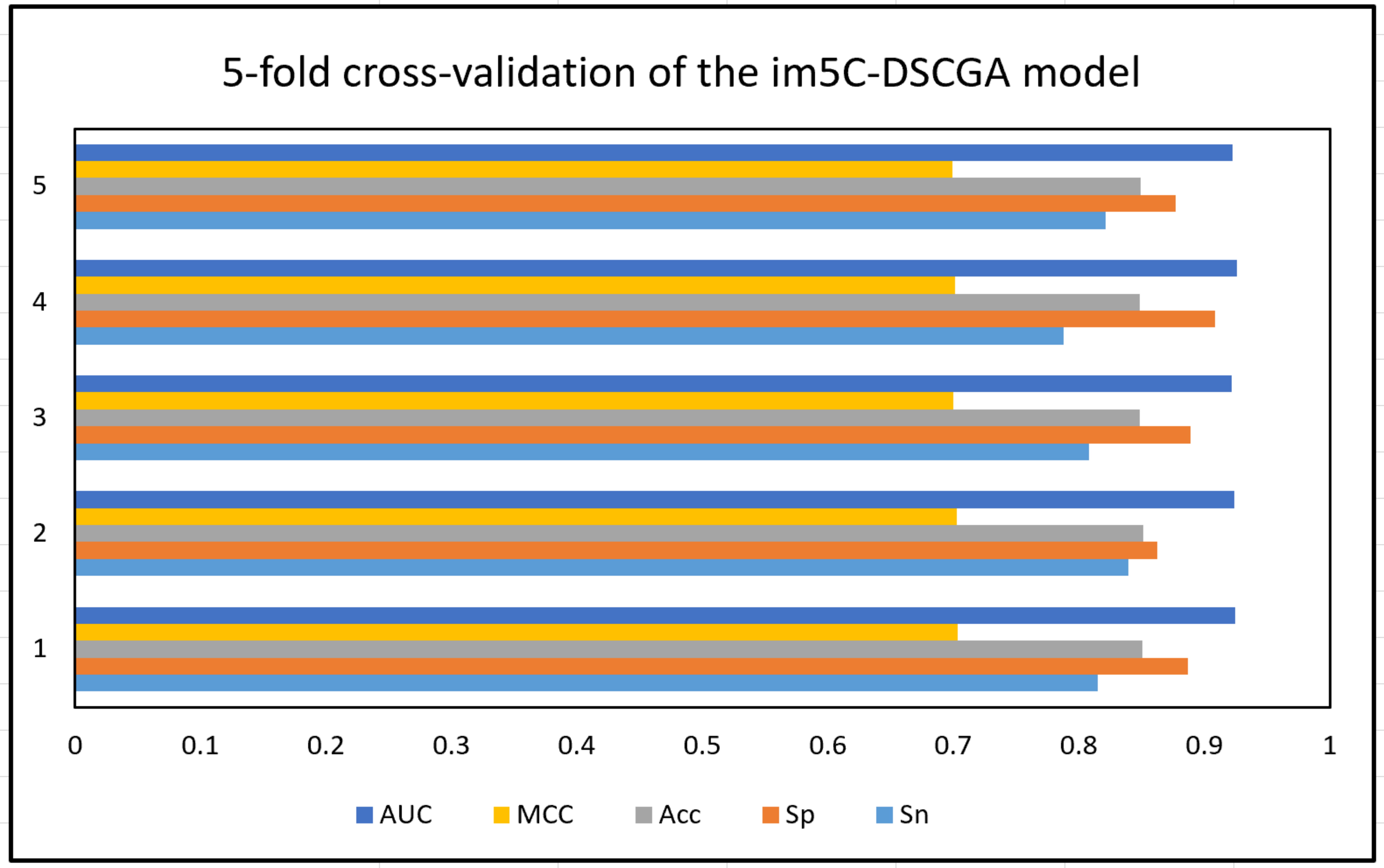Fig. 20.

Performance of im5C-DSCGA model on five-fold cross-validation.

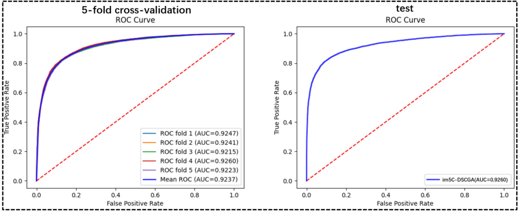Fig. 21.

Performance of im5C-DSCGA model.

Using the im5C-DSCGA network framework proposed in this work, we compared the performance of five different feature encoding methods, including one-hot, one-hot + NPF, one-hot + ND, NPF + ND, and one-hot + NPF + ND. They encode RNA sequences into 4 $\times$ 41, 7 $\times$ 41, 5 $\times$ 41, 4 $\times$ 41, and 8 $\times$ 41 feature matrixes, respectively. Thereafter, these five encoded generated feature matrices were inputted into the im5C-DSCGA network framework, and the experimental results on the five-fold cross-validation and independent tests are displayed in Fig. 22, respectively.

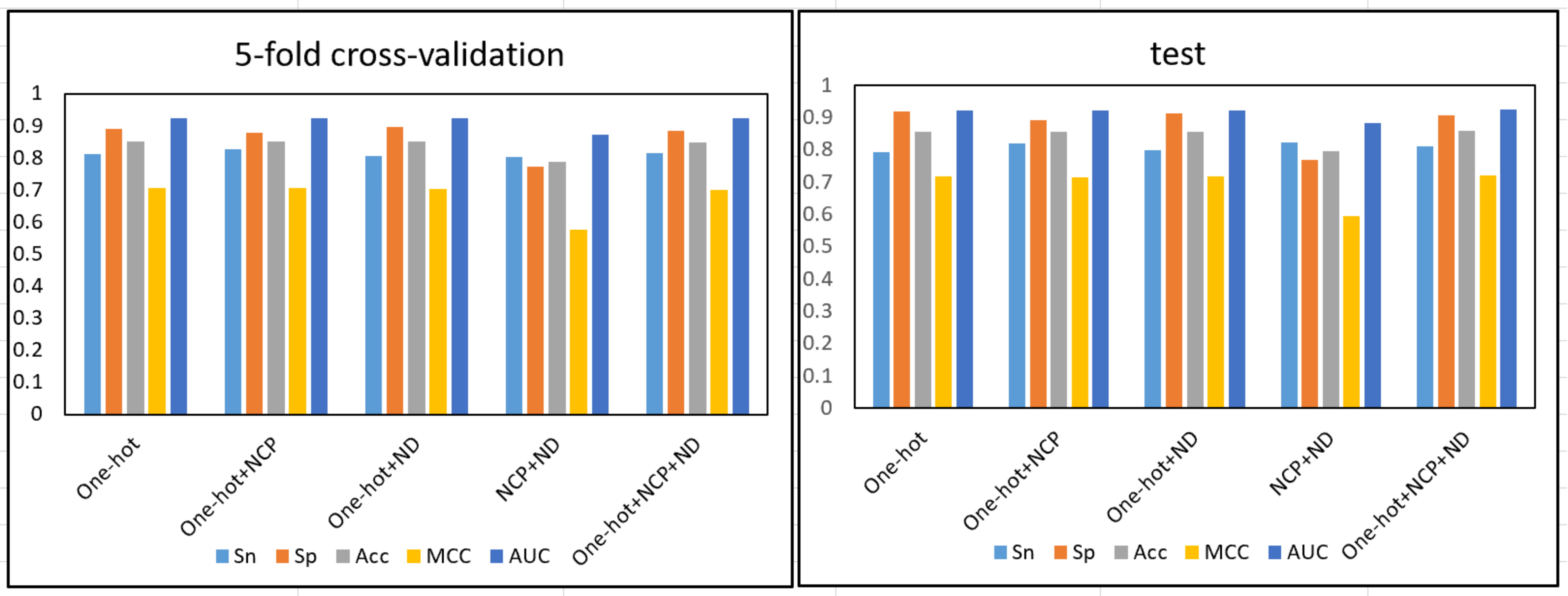Fig. 22.

Ablation experiment of feature encoding method.

It can be distinctly seen that the four feature encoding methods, one-hot, one-hot + NPF, one-hot + ND, and one-hot + NPF + ND, significantly outperform the NCP + ND feature encoding. However, the feature encoding for the one-hot + NPF + ND combination outperformed the feature encoding for the other combinations, in terms of MCC performance evaluation metrics. Therefore, we adopted the one-hot + NPF + ND feature encoding as the final feature encoding method for the im5C-DSCGA network framework.