GpemDB: A Scalable Database Architecture with the Multi-omics Entity-relationship Model to Integrate Heterogeneous Big-data for Precise Crop Breeding

^*Correspondence: gongliang_mi@sjtu.edu.cn (Liang Gong); chlliu@sjtu.edu.cn (Chengliang Liu)
^†These authors contributed equally.
Academic Editor: Tatsuya Akutsu

Front. Biosci. (Landmark Ed) 2022, 27(5), 159; https://doi.org/10.31083/j.fbl2705159

Submitted: 21 December 2021 | Revised: 25 March 2022 | Accepted: 24 April 2022 | Published: 17 May 2022

(This article belongs to the Special Issue Selected Papers from the 12th International Conference on Bioscience, Biochemistry and Bioinformatics (ICBBB 2022))

This is an open access article under the CC BY 4.0 license.

Download PDF

Brower Figures

Cite

Abstract

Background: With the development of high-throughput genome sequencing and phenotype screening techniques, there is a possibility of leveraging multi-omics to speed up the breeding process. However, the heterogeneity of big data handicaps the progress and the lack of a comprehensive database supporting end-to-end association analysis impedes the efficient use of these data. Methods: In response to this problem, a scalable entity-relationship model and a database architecture are firstly proposed in this paper to manage the cross-platform data sets and explore the relationship among multi-omics, and finally accelerate our breeding efficiency. First, the targeted omics data of crops should be normalized before being stored in the database. A typical breeding data content and structure is demonstrated with the case study of rice (Oryza sativa L). Second, the structure, patterns and hierarchy of multi-omics data are described with the entity-relationship modeling technique. Third, some statistical tools used frequently in the agricultural analysis have been embedded into the database to help breeding. Results: As a result, a general-purpose scalable database, called GpemDB integrating genomics, phenomics, enviromics and management, is developed. It is the first database designed to manage all these four omics data together. The GpemDB involving Gpem metadata-level layer and informative-level layer provides a visualized scheme to display the content of the database and facilitates users to manage, analyze and share breeding data. Conclusions: GpemDB has been successfully applied to a rice population, which demonstrates this database architecture and model are promising to serve as a powerful tool to utilize the big data for high precise and efficient research and breeding of crops.

Keywords

database

multi-omics

phenomics

metadata-level

informative-level

visualization platform

big data

crop

precise breeding

rice

1. Introduction

There lies a continuing demand for agriculture to reinvent itself, striving for better agronomic performances such as enhanced productivity, cost-efficiency, and crop quality. Varieties need to combine a lot of excellent traits that help to against a multitude of stresses, ensure crop uniformity and storability. Traditional breeders attempt to combine these traits by methods which rely on random genome modifications such as biparental cross, chemical mutagenesis, and $\gamma{}$ -radiation mutagenesis and so on. However, these traditional breeding methods are usually time-consuming and labour-intensive, because their screening often relies on manual measurement of a single trait. When we perform genomic selection, we need more detailed information on the crops, not only one trait but also many other phenotypes at the same time. Phenomics is a good way to solve this problem, by phenotyping a large number of individuals for a great number of traits throughout the development of the plants, in a non-destructive manner and with good accuracy.

Nowadays, plant phenomics has produced massive data involving millions of images and other information from different sensors and scales performed in the field and in controlled conditions, concerning hundreds of genotypes at different phenological stages and management methods [1]. Therefore, they often also involve multi-omics data associated with genomic, enviromics and management information. For most researchers, this huge data is extremely expensive and difficult to analyze and manage. Hence, there is an increasing need to make them available to a range of users openly, allowing re-analyses and upload or download our data freely. A database containing multi-omics data and statistic tools is a good way to solve this problem.

Database architecture have proved to be effective in the studies of genomics and phenomics.For example, in the filed of human disease research, FBN1 genetic testing is key to establishing a clinical diagnosis of Marfan syndrome, and FBN1 databases (http://www.umd.be/FBN1/) are often used to evaluate variant causality. Kristian et al. [2] evaluated the current databases regarding FBN1 variants, validated the associated phenotype records with a new Marfan syndrome geno-phenotyping tool, and quantified the association of FBN1 variants with Marfan syndrome phenotypes. Likewise, gene-phenotype association databases can also be used in plants. Experiment-driven database analysis is employed in forward genetics to predict the function of genes associated with a mutant phenotype [3]. TropGeneDB (http://tropgenedb.cirad.fr) is a web database that manages genomic, genetic, and phenotypic information on tropical crops [4]. Another database for the management of phenotype information called J-phenome was also developed [5]. The OsGDB is being developed as a part of the NSF-funded project, supporting cyberinfrastructure for plant genome research [6]. Therefore, we hope to use the gene-phenotype association database for crop breeding.

Furthermore, using deep learning techniques to predict phenotype from gene expression data has become a reality in big data [7]. Deep learning algorithms often rely on a large amount of data, so it is necessary to build a database. EURISCO (http://eurisco.ecpgr.org) collects data on crops preserved by nearly 400 institutes in Europe and outside Europe, protecting the world’s agricultural biodiversity [8]. However, it is currently limited to collecting data in a non-native environment and saving it into the database and cannot import heterogeneous big data. GnpIS (http://urgi.versailles.inra.fr/gnpis) is an information system integrating genetic and genomic data of plants and fungi [9]. As a plant database, it integrates genetic information and genomic data. But it’s not very scalable. Optimas-DW (http://www.optimas-bioenergy.org/optimas_dw) is a comprehensive database of maize transcriptomics, metabolomics, ionomics, proteomics and phenomics [10]. The database contains a richer variety of data to analyze the impact of specific environmental conditions or developmental stages on maize. But it doesn’t have any plugin. MBKbase (www.mbkbase.org) is an integrated omics knowledge base for rice breeding [11]. It integrates rice germplasm resource information, multiple reference genomes, unified gene loci, typical data, known alleles and expression data, and can visually display the relationship between genotype and phenotype. However, we hope to integrate more kinds of plant information (such as the Environmental and Management factors in GpemDB) into the database to help breeding.

However, there are still some defects in the previous databases. Some Genome databases have the function of automatic gene screening, however usually lack the ability of statistical analysis like variance and correlation analysis [12]. Some databases for phenomics didn’t support complex analysis involved in precise breeding [13]. Although some scholars have integrated some phenotypic data, such as PHIS (Phenotyping Hybrid Information System) [1], Planteome [14] and AtMAD (Arabidopsis thaliana multi-omics association database) [15], they didn’t take into account sufficient factors which are necessary for crop breeding. Furthermore, understanding intrinsic interactions of phenotype, genotype, environment, and management is vital for breeding new cultivars and farming systems [16], unfortunately, there are rare crop databases containing and associating all those four types of big data.

As rice is the staple food of more than half of the world’s population [17], this article selected rice as the object of the case study. Traditional research on rice breeding focused on conventional phenotypic traits and could not keep up with global climate change and rapid development of genomic technology together with agricultural management technology. A more complete database involving genomic, environmental, phenotypic and managerial factors needs to be established for further improving rice breeding and building a breeding platform with high precision, automation and throughput [18].

The paper is organized as follows. Section 2 demonstrates the crop factors for breeding. Four types of data structure (genomics, phenomics, enviromics, management) are designed, and the heterogeneous data involved in four dimensions was integrated. Section 3 builds an entity-relationship model for describing the breeding traits and their linkages. In Section 4, some frequently-used statistic tools are added to the database to facilitate crop research. In Section 5, we establish a metadata-level layer to store the raw multi-omics data and an informative-level layer to store the processed data for end-to-end queries in different applications. Then a visualization platform is developed to display the content of the database in Section 6. Finally, a case study using some old data has proved this database is useful and efficient for crop research and breeding.

2. Materials and Methods

2.1 Crop Factors

It is very common to use multi-omics data to participate in breeding, but there is no database that integrates all four omics information of gene, phenotype, environment, and management into one platform. Here, we presented some traits that matter greatly in traditional rice breeding. To get these traits, we should design some complex experiments, like choosing appropriate materials and cultural environments, giving good treatment and management. Therefore, any trait actually contains much other information that has been rarely used in traditional crop breeding. In this study, we hope to make full use of all the factors that may influence these traits.

In traditional breeding, we are usually concerned with the relationship between only one factor with the target trait, like genotype with the trait, or treatment with the trait. In this study, we try to improve the compatibility of heterogeneous data and integrate all the factors together, and then make a comprehensive analysis and use of all these data, and finally enhance our research and breeding.

2.1.1 Genomic

Genotype has important effects on phenotype [19]. Through QTL mapping and GWAS analysis, it’s easy to quantify the effect of genotype on phenotype in crop breeding. In recent years, with the development of high-throughput DNA sequencing technology, the accuracy and efficiency of genotyping have been greatly improved and the cost of sequencing has been dramatically reduced. In addition, linkage analysis is one of the most powerful methods to find the type and location of genes that significantly influence phenotypic traits. As a result, using such linkage analysis to explore important agricultural genes has been widely used in almost all plant species. For instance, a lot of studies on genes that may affect yield, resistance to biotic/abiotic stress, grain quality and so on have been conducted in the past years [20]. The genetic sequence data are indispensable for modern crop improvement.

Besides the genotype, the information of gene expression, even the quantity and type of proteins and metabolites all greatly influence a plant’s phenotype. Because genotype, gene expression, protein, and metabolites are all refer to the intrinsic and autogenous factors of the plants, we put these four type omics data together in the name of genomics. Furthermore, there have been a lot of good online databases serving for genes, mRNAs, proteins, and metabolites searching and downloading. In our database, we set several linkages with some existing databases that are often used in crop research. All this information could be linked to each other by the name of varieties and genes, finally, we set a general template, including the four major entities of genomics and the database parameters corresponding to each entity, as shown in Table 1.

Table 1.Genomic factors.

Entity		Database parameters
Genome	Gene	Sequence	SNP	Chromosome Location
Transcriptome	Gene	Sequence	Expression	Tissue and organ	Treat
Proteome	Gene	Sequence	Expression	Tissue and organ	Modification
Metabolome	Gene	Expression	Tissue and organ	Treat

2.1.2 Phenomic

Phenotype is the most direct indicator of crops’ breeding potential and characters. According to the data format, it is divided into two categories, one is non-image trait that most of the traditional traits belong to this type like plant height and weight, and the other is image trait usually called i-trait from all kinds of images from short wave to long wave. Then according to different spatial scales, phenomics encompasses many categories. In individual plants, there are different organs including root, stem, leaf, grain, spike phenotypes. For example, grain size [21], leaf size [22], stem diameter [23] and other important agronomic traits. In a whole plant, plant height, tillers number and heading date are always concerned mostly. In the plot of plants, the phenotypes of the canopy like canopy color, size and temperature are often concerned. Table 2 includes common entities of plant phenotyping and database parameters corresponding to each entity.

Table 2.Phenotyping factors.

Entity	Database parameters
Root	RL	RN	EA	RA	RT
Stem	SD	SL	SLA
Leaf	FLA	FLS	LCC
Grain	GN	AGL	AGL	1000GW	GAR
Spike	SIN	SL	SIL	PT	PC
Plant	TN	PH	HD
Canopy	CG	CF	CS

With the fast development of phenomics, millions of raw images from different sources (like RGB, hyper-spectrum, infrared and radar) have been produced. They can be transferred into traditional digital traits through professional analysis. But for most of biologists and breeders, it is hard to develop a specific software to deal with such huge raw image data by themselves. So, we set an entity for different raw images input as shown in Table 2. Users can upload their own raw images into this database freely, which not only helps users to manage their data but also will help them to analyze these huge data. In the future, we plan to develop some tool kits to deal with some specific raw image data automatically in this database. We elaborate on this in Section 2.3 of this paper.

2.1.3 Enviromic

With the change of global climate, the influence of the environment on crops is more and more evident, usually causing serious yield loss [24, 25, 26]. In order to increase rice yield, the effects of environmental factors on rice breeding need to be quantitatively analyzed. Table 3 includes the common natural environment factor entities (such as water, soil, light, air, and geolocation) related to plant growth in the database and the database parameters corresponding to each entity.

Table 3.Environmental factors.

Entity	Database parameters
Light	LI	IT
Soil	ST	STe	SF	SpH	SSa	SH
Air	AT	AH	AP	CO2	O2	N2	SO2
Water	WT	Pr	WpH
Geolocation	GPS

2.1.4 Management

Management could also affect rice yield seriously [27], therefore it’s necessary to be included in the database as an essential part. Management factors include fertilization, irrigation, and planting methods, like fertilizer types, amounts, time and intervals, irrigation amounts and time, hot or drought treatment, and the information of the apparatus used to obtain images (Table 4).

Table 4.Managing factors.

Entity	Database parameters
Apparatus	AN	AM	AS	AP
Fertilization	FTs	FT	FA	FI
Irrigation	IT	IA	II
Planting method	T	PD	In	He	Di

2.1.5 Heterogeneous Data Integration

Each data we get in experiments may contain 4 types of information, including its phenotype, genotype, environmental condition, and the way of management. The data are heterogeneous because of different sources and different data structures. For example, genomic data include gene sequences, SNP format, etc., phenotypic data include image format, infrared spectra, manually recorded data, etc., environmental data include arrays obtained from sensors, point cloud data, etc., and management data include csv format.

Therefore, the ability of the database to be compatible with heterogeneous data is very important. We integrated these heterogeneous data by their relationships like some common items. For example, the plant number may occur in all four categories’ data, so we use the multi-features joint primary key (e.g., test batch-growing area number-plant number) to combine all these data together. “Entity” is a name of the data table, and hundreds of such tables make up the database. “parameters” is the content of the entity table, and one entity table can have many parameters. And some parameters may have secondary parameters, like genomic (Table 1) that has a lot of secondary parameters like genes name, position, length, function and so on. Users can retrieve the parameters to get the information they are interested in.

2.2 Entity-Relationship Models of Multi-omics Data

2.2.1 Introduction to ERM

The Entity-relationship model, put forward by P.P.Chen in 1976 [28], was an efficient method used to design database schema in different subjects, such as internal control construction of a transaction system [29], data storage service for web-based, data-oriented collaboration [30] and a system of adult extended education [31]. Although improved entity-relationship models have been put forward [32, 33, 34, 35], it is more convenient to directly modify the rules of the basic entity-relationship model in this article. In the entity-relationship model, study subjects can be divided into two classifications containing entities and relationships. An entity is a real-world object with some attributes. Plant breeding traits are defined as entities within our methodology. A relationship is an association among entities, which can be used to link the four omics according to the entities. A relationship is a mathematical relation among n entities and each taken from an entity set.

(1) $\left\{\left[e_{1},e_{2},\cdots,e_{n}\right]\mid e_{1}\in E_{1},e_{2}\in E_{2}% ,\cdots,e_{n}\in E_{n}\right\}$

Each tuple of entities, [e ${}_{1}$ , e ${}_{2}$ , …, e ${}_{n}$ ], is a relationship.

Every entity can be transformed into a table in the database, and each parameter of the entity becomes a field in the corresponding table. ERM can automatically generate entity-relationship diagrams [36] and simplify the structure of the database for breeding.

However, traditionally an ERM only possesses the relationship of 1:1 and 1:M, which could not distinguish the relationship between two entities with multi-omics data. Hence we propose a mapping process to realize the M:N association among entities, as explained in Section 5.4 in detail. In this way, the database is more scalable.

2.2.2 ERMs of Multi-Omics Data

As the ERMs are numerous, one example of an image-related entity-relationship model is shown below in Fig. 1. Analysis of images is an effective and important way to precisely describe most phenotypes [36, 37, 38, 39, 40, 41, 42]. Thus, it is necessary to illustrate the relationship between images and common entities.

Fig. 1.

Image-related entity-relationship model.

Images have many attributes such as resolution and content. Therefore, fields named “resolution” and “content” will be added to the table named “Image”. Similarly, in the corresponding tables, the name of the field will be called, for example, attributes of root, stem and other organs. Every organ corresponds to a variety of images so that the relationship between images and organs is N:1.

2.3 GPEMDB Analysis Plug-in

Traditional feature engineering is based on a few explicit features (such as plant height, leaf length, etc.), using variance analysis, information entropy increase, etc. for analysis. In combination with big data, many implicit features can be used, such as using deep learning technology to extract convolution kernel features. Here, we insert some statistic tools into the database, so users could analyze data in the database directly, like anova, sorting, correlation, and parametric test. Users can also use some deep learning tools, such as powdery mildew recognition model [43] and rice point cloud segmentation model [44], etc. The toolkit accesses the database through the API. The statistics are calculated and displayed after the tool is called. Therefore, GPEMDB is not only a storage of big data of agriculture, but also a useful tool to analyze data, which enhances the power and utility of the database.

Additionally, it is also friendly for raw image data. The user first needs to manually configure the the image-acquiring settings, which will be saved to the database. Before the image is stored in the database, the database will automatically standardize the image (scaling, rotation, segmentation, etc.) according to the configured parameters.

2.4 GpemDB Database Construction

2.4.1 Overall Dataflow of Rice Breeding Information Processing

The GPEM database was designed to support the application of crop research and breeding. It includes two layers: the metadata-level layer and the informative-level layer. The metadata-level layer is constructed based on the entity-relationship model and contains original data. The informative-level layer is based on the metadata-level layer and is designed to support end-to-end queries. Different applications have the same metadata-level layer, but the informative-level layers are customized differently. No application uses the data of the metadata-level layer. Even if the application intends to obtain the original data when acquiring the data, it still needs to pass the informative-level layer to implement the same calling rules. The dataflow is shown in Fig. 2. The collected raw data is stored in the metadata layer after classification and association, and the data in the metadata-level layer reaches the informative-level layer after data processing or batch processing. The difference between data processing and batch processing is that data processing is a call-time operation, while batch processing is applicable to the access of hot data, i.e., the results are stored in advance batch processing for quick access. Finally, the user gets the desired plant data in the informative-level layer.

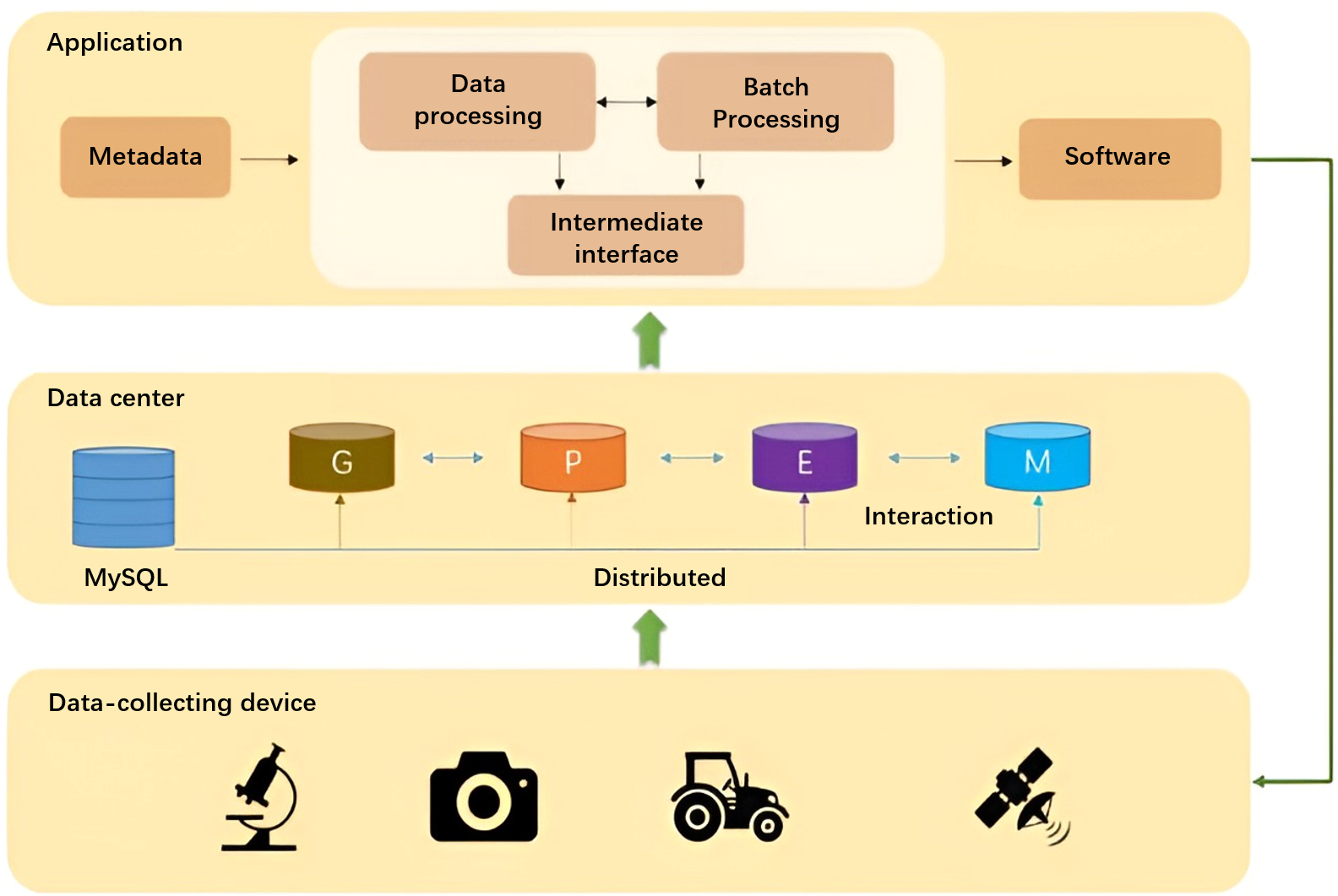Fig. 2.

Dataflow of rice breeding.

The raw data is either entered manually or read automatically by the instrument, and our proposed database architecture supports both data sources. We provide an interface for the database through ODC (Open Database Connectivity). Data is stored in the metadata-level layer of the GPEM database through a specific interface. The original data can be processed and then stored in the informative-level layer which will be directly accessed by applications. The functions and usage flow of the database we envision are shown in the Supplementary Fig. 1 and Supplementary Fig. 2.

2.4.2 Metadata-level Layer Based on the Entity-relationship Model

Table 5 and Table 6 are converted from the ERM displayed in Fig. 1. Table 5 shows the entities included in the plant phenomics database and the parameters corresponding to each entity. In the database we establish relationships between different tables through a relationship table (Table 6). All the tables and fields in the database can be generated in this way.

Table 5.Entities to tables.

Table name	Fields
Root	ID	RL	RN	EA	RA	RT
Stem	ID	SD	SL	SLA
Leaf	ID	FLA	FLS	LCC
Grain	ID	AGL	AGW	1000GW	GN	GAR
Spike	ID	SIN	SL	SIL	PT	PC
Plant	ID	PS	PH
Image	ID	IR	IC	IDIM	IF	IT

Table 6.Relationships to tables.

Table Name	Fields
Image_root	Image ID	Root ID
Image_stem	Image ID	Stem ID
Image_leaf	Image ID	Leaf ID
Image_grain	Image ID	Grain ID
Image_spike	Image ID	Spike ID
Image_plant	Image ID	Plant ID

2.4.3 Informative-level Layer

The informative-level layer exists in the same database as the metadata-level layer. This layer seems to be redundant, as users can extract data directly from the metadata-level layer and then conduct calculations. However, directly extracting data from the underlying layer requires complicated operations. The informative-level layer helps to reduce the frequency and complexity of data acquisition from the underlying layer. Users can also define customized informative tables which ensure them to acquire data directly instead of through complicated relationships.

Table 7 shows the new table format required in a spike analysis example. Some analyses of traits need image processing, especially in the field of machine learning [45], so the following three tables will be necessary.

Table 7.Tables related to the analysis of spike.

Table name	Fields
Spike	ID	SIN	SL	IL	PT	PC
Image	ID	IC	IDIM	IT	IR	IF
Image_spike	Image ID	Spike ID

Analysis of the spike needs image data in the “image” table. Image ID needs to be matched with the corresponding Spike ID. Then image data can be acquired according to Image ID. However, this process involves at least three tables, and if a type of spike is to be analyzed, more data tables will be necessary. Therefore, a table named “spike_analysis” can be added to the database as shown in Table 8, so that only one table is needed. QL means quality level. TI means typical image. AGS means the average number of grains within spikes of this type.

Table 8.“spike_analysis” table.

Table name	Fields
Spike Analysis	Spike type ID	QL	TI	AGS

2.4.4 Scalability of GpemDB

Scalability mainly refers to the supplement of the database’s structure without disrupting the structures of existing data tables.

(1) Add new Entities. Take “ideotype” [46] as an example.

Firstly, add a table named “ideotype” and assign it to the “Phenotyping” class. Secondly, find all the existed related entities of ideotype such as virtual colony. Thirdly, add a table named “virtual_colony_ideotype”, with fields named “virtual_colony id” and “ideotype id”, and assign it to the “Relationship” class. The format of the new entity table is shown in Table 9. In this way, it is not necessary to modify the existing data tables.

Table 9.Ideotype-related tables.

Table name	Fields
Ideotype	Ideotype ID	IPH	ILA	ITN
Virtual_colony_ideotype	Virtual_colony ID	Ideotype ID

(2) Add new attributes. Take “plant” as an example.

Table 10 shows a comparison of newly created attributes in a table. The original attributes of the plant are site (of growth) and plant height as shown in the second row of Table 10. If new attributes, lodging resistance (PLR) and growth cycle (PGC), are added to the existing entity, the table will be as shown in the third row of Table 10. Meanwhile, other tables are related to this table by the means of the key. Therefore, the new attributes are also accessible in other related data tables.

Table 10.Add new attributes.

Table name	Fields
Plant (before)	ID	PS	PH
Plant (after)	ID	PS	PH	PLR	PGC

2.4.5 Visualization Platform

There are many visualization platforms for managing databases. However, the platforms are either charged, such as Navicat for MySQL, or too complicated, such as MySQL Workbench. Therefore, many specific software platforms are designed for the study of plants [47, 48, 49]. In this paper, to simplify the management of the GPEM database, a specific visualization platform was developed (Fig. 3). This software consists of two parts, the metadata-level part and the informative-level part.

Fig. 3.

visualization platform. (A) Metadata-level user interface. (B) Informative-level user interface. (C) Metadata-level operation. (D) Informative-level operation.

The main interface displays the list of names of data tables in the database according to their classifications. The metadata-level part includes five subparts that are Genotyping, Envirotyping, Phenotyping, Management and Relationship, constructed based on the entity-relationship model. The informative-level part includes two subparts, which are the regular analysis part for users to add customized tables, and the image process part for users that focus on machine learning.

The “operation” button can be clicked to enter the corresponding sub-interfaces. In the metadata-level part, users can add and delete fields in existed tables as well as add new tables in the database. However, original data is not accessible here because the amount of data is too large. In the informative-level part, users can also modify fields in existing tables as well as add new tables.

2.5 Case Study

A natural population comprising 4 Aus, 154 Indica and 107 Japonica rice accessions from the mini-core collection of Chinese rice germplasm and a core drought-resistance rice germplasm collection are used for the case study (Table 11, Ref. [50, 51, 52]). There are four types of information of this population including genotype, phenotype, environment, and management. First, this population had been re-sequenced in the Illumina Sequencing Platform in 2011, and 3038555 SNPs of the population were extracted for further analysis. Second, using this population, 4 different experiments were carried out in different environments and managements. Third, there are 2 types of phenotyping data: one is raw image data which can be acquired from the high throughput phenotyping platform (Fig. 4) and the other is traditional quantitative data. The images were stored in the format of picture (jpg) in the raw image entity. The digit data were measured manually and showed in digital numbers as the traditional agronomic traits. Totally, we imported 12 digital traits including leaves area (LA), Plant height (PH), Tiller number (TN), Deep roots number (DR), Shallow roots number (SR), Total roots number (TR), Ratio of deep roots (RDR), Roots per tiller (R/T), Growth speed of seminal roots (GSR), Gravitropic response speed of seminal roots (GRSS), Mesocotyl length of rice seedlings in dark germination (MLw in water and MLs under 5 cm sand culture); and some RGB pictures of 16 rice accessions from the big population. To get the details of the experiments could refer to the related references in Table 11.

Table 11.The information list of rice traits used for the case study.

Genotype	Phenotype		Environment		Management	Reference
3038555 SNPs	Images	Quantitive traits	Location	Time
	RGB	LA	Shanghai, lab	2019	Paper bag	unpublished
		PH	Hainan, filed	2013	Basket method	Lou et al., 2015 ${}^{1}$ [50]
		TN	Hainan, filed	2013	Basket method	Lou et al., 2015 ${}^{1}$ [50]
		DR	Hainan, filed	2013	Basket method	Lou et al., 2015 ${}^{1}$ [50]
		SR	Hainan, filed	2013	Basket method	Lou et al., 2015 ${}^{1}$ [50]
		TR	Hainan, filed	2013	Basket method	Lou et al., 2015 ${}^{1}$ [50]
		RDR	Hainan, filed	2013	Basket method	Lou et al., 2015 ${}^{1}$ [50]
		R/T	Hainan, filed	2013	Basket method	Lou et al., 2015 ${}^{1}$ [50]
		GSR	Shanghai, lab	2018	0.8% Agrose plate	Lou et al., 2021 ${}^{2}$ [51]
		GRSS	Shanghai, lab	2018	0.8% Agrose plate	Lou et al., 2021 ${}^{2}$ [51]
		ML	Shanghai, lab	2013	MLw	Wu et al., 2015 ${}^{3}$ [52]
		ML	Shanghai, lab	2013	MLs	Wu et al., 2015 ${}^{3}$ [52]

Fig. 4.

High throughput phenotyping platform. (A) Side view. (B) Front view.

3. Results

3.1 Analysis of Variance

Using the database GpemDB can help us to manage and analyze large amounts of data much more conveniently and efficiently. For example, when we look at the variation of TN (tiller number) in the population, it is surprised to find the least ten accessions are all japonica rice, while most of the top ten (80%) are indica rice. The TR (total roots number) also has the same trend as TN: 9/10 of the least TR accessions are japonica rice, while 9/10 of the top ten are indica rice. These results give us a hint that some agronomic traits may have a great differential between the two subspecies of japonica and indica. The indica and japonica are two main subspecies of Asia cultivated rice, and they evolved from different environments and evolved to different characters what are very important for research and breeding.

Firstly, we calculated the average of all traits both in Indica and Japonica groups by correlating them through the relationship shown in Fig. 5. Secondly, we can use Eqn. 2 to do t-test of the traits between Indica and Japonica.

(2) $t=\frac{m_{A}-m_{B}}{\sqrt{\frac{s_{A}^{2}}{n_{A}}+\frac{s_{B}^{2}}{n_{B}}}}$

Fig. 5.

Relationship between traits in GpemDB.

m ${}_{\text{A}}$ represents the average value of A, m ${}_{\text{B}}$ represents the average value of B, S ${}_{\text{A}}$ ${}^{2}$ represents the variance of A, S ${}_{\text{B}}$ ${}^{2}$ represents the variance of B, n ${}_{\text{A}}$ represents the number of A samples and n ${}_{\text{B}}$ represents the number of B samples.

Finally, we can get the difference of 11 traits between the japonica group and the indica group (Table 12). Both MLw and MLs are significantly different between the two subspecies, and the japonica varieties usually have longer mesocotyl length than the indica, especially under the culture of sand. In the 0.8% Agrose plate, indica varieties’ seminal root responds to gravity much more quickly than japonica (GRSS), and they also with higher growth speed compared with japonica. Using the method of basket, the TN, SR, TR and RDR show a great difference between indica and japonica, that indica varieties have larger TN, SR and TR than japonica, while japonica has better RDR.

Table 12.The comparison result of 11 agronomic traits between indica and japonica subspecies.

Subspecies	Indica	Japonica	t-test
Amount	154	107
MLw (mm)	3.62	5.52	3.65E-02*
MLs (mm)	3.05	5.45	3.11E-06**
GRSS (°/h)	42.49	39.71	1.57E-03**
GSR (mm/h)	0.04	0.03	1.99E-03**
PH (cm)	88.29	90.83	0.153
TN	44.2	31.21	5.32E-21**
DR	98.37	90.59	0.152
SR	261.72	163.78	1.77E-20**
TR	449.61	316.1	6.13E-16**
RDR	0.22	0.29	2.65E-11**
R/T	10.45	10.91	0.332
Note: Mesocotyl length of rice seedlings in dark germination in water (MLw) and under 5 cm sand culture (MLs)PH; GRSS, Gravitropic response speed of seminal roots; GSR, Growth speed of seminal roots; Plant height; TN, Tiller number; DR, Deep roots number; SR, Shallow roots number; TR, Total roots number; RDR, Ratio of deep roots; R/T, Roots per tiller. * shows the difference is significant at p $<$ 0.05, ** shows the difference is very significant at p $<$ 0.01.

3.2 Analysis of Correlation

Furthermore, in this database we can use Eqns. 3,4,5 to analyse the correlation among these traits since some of them always shows the same trends.

(3) $r(X,Y)=\frac{{Cov}(X,Y)}{\sqrt{{Var}[X]{Var}[Y]}}$

(4) ${Cov}({X},{Y})=\frac{\sum_{i=1}^{n}\left(X_{i}-\bar{X}\right)\left(Y_{i}-\bar{% Y}\right)}{n-1}$

(5) ${Var}(X)=\frac{\sum_{i=1}^{n}\left(X_{i}-\bar{X}\right)^{2}}{n-1}$

r(X,Y) represents the correlation coefficient of X and Y, Cov(X,Y) represents the covariance of X and Y, Var[X] represents the sample variance of X.

Not surprisingly, a lot of traits correlate closely with each other (Table 13). For example, MLw and MLs have a good positive relationship with a large correlation index at 0.78, which suggested the mesocotyl length of rice may have high heritability and it may be mainly decided by the genetic factor but not the environment. This trait also correlates with PH and R/T positively, but negatively with GSR and TN. These results had never been reported in other papers. From these results, we can get some enlightenment for researchers and breeders. To breed a new variety with long mesocotyl length for direct seeding on dry land, we’d better choose the materials having higher height, fewer tillers and slower growth of the seminal root.

Table 13.The correlation between the traits.

	MLw	MLs	GRSS	GSR	PH	TN	DR	SR	TR	RDR
MLs	0.78 ${}^{**}$
GRSS	0.00	–0.10
GSR	–0.23 ${}^{**}$	–0.21 ${}^{**}$	0.22 ${}^{**}$
PH	0.32 ${}^{**}$	0.45 ${}^{**}$	0.03	–0.05
TN	–0.23 ${}^{**}$	–0.36 ${}^{**}$	0.13 ${}^{*}$	0.20 ${}^{**}$	–0.15 ${}^{*}$
DR	0.06	0.03	0.15 ${}^{*}$	–0.04	0.13 ${}^{*}$	0.07
SR	–0.06	–0.17 ${}^{**}$	0.09	0.15 ${}^{*}$	0.01	0.50 ${}^{**}$	0.30 ${}^{**}$
TR	–0.03	–0.13 ${}^{*}$	0.13 ${}^{*}$	0.12	0.06	0.46 ${}^{**}$	0.57 ${}^{**}$	0.95 ${}^{**}$
RDR	0.08	0.16 ${}^{*}$	0.05	–0.15 ${}^{*}$	0.09	–0.35 ${}^{**}$	0.61 ${}^{**}$	–0.50 ${}^{**}$	–0.24 ${}^{**}$
R/T	0.22 ${}^{**}$	0.26 ${}^{**}$	0.01	–0.09	0.21 ${}^{**}$	–0.47 ${}^{**}$	0.52 ${}^{**}$	0.43 ${}^{**}$	0.53 ${}^{**}$	0.13 ${}^{*}$
Note: Mesocotyl length of rice seedlings in dark germination in water (MLw) and under 5 cm sand culture (MLs)PH; GRSS, Gravitropic response speed of seminal roots; GSR, Growth speed of seminal roots; Plant height; TN, Tiller number; DR, Deep roots number; SR, Shallow roots number; TR, Total roots number; RDR, Ratio of deep roots; R/T, Roots per tiller. * shows the difference is significant at p $<$ 0.05, ** shows the difference is very significant at p $<$ 0.01.

3.3 Analysis of Genetic Information

Using this database of GpemDB, we can also easily find genetic information of the accessions in which we are interested. Dro1 is the first deep rooting gene that had been cloned in rice and proved to affect the root architecture significantly [53]. Its ORF has a single 1-bp deletion within exon 4 in IR64 compared with KP accessions, which will result in the introduction of a premature stop codon. We are interested in the varieties with extreme RDR in this population that would contain this functional SNP. Therefore, we extracted all the SNPs of the gene Dro1(Os09g043980040/LOC_Os09g26840.1) in 20 accessions with the highest and least RDR. The 10 top RDR varieties are named as H group with an average of RDR up to 48%, and the 10 least RDR varieties named as L group with the average of RDR at 11% (Table 14). This gene has 5 CDSs, but no SNP has been found on the CDS region in this population. In the other parts of the gene including promoter, 3UTR, introns and 5UTR, there are 23 SNPs with different types of alleles. The SNP difference of the alleles in Intron2 is notable.

Table 14.SNP polymorphism in the gene DRO1 and comparison between deep rooting and shallow rooting cultivars.

Gene elements	Position	SNP name	Alleles in H group ${}^{a}$	Alleles in L group ${}^{b}$
Three prime UTR2	16307780—16308009	NA
Three prime UTR1	16308120—16308152	NA
CDS5	16308153—16308172	NA
CDS4	16308269—16308440	NA
CDS3	16308532—16309010	NA
Intron2	16309011—16310370	916309309	10G	10G
		916309349	10C	10C
		916309459	10C	7C/3T
		916309742	10G	7G/3A
		916310217	8C/2T	6T/4C
CDS2	16310374—16310452	NA
Intron1	16310453—16310568	916310551	8G/2A	10G
CDS1	16310569—16310574	NA
Five prime UTR	16310575—16310837	916310688	5A/5G	6A/4G
Promoter	1631087+2Kb	916310954	9G/1T	7G/2T
		916311266	10T	10T
		916311280	8C/2A	10C
		916311303	9C/1T	7C/3T
		916311313	10C	10C
		916311348	10A	10A
		916311387	10C	10C
		916311467	10T	10T
		916311512	10C	10C
		916311633	5G/5A	6G/4A
		916312351	5G/5T	6G/4T
		916312455	8G/2C	6G/3C
		916312587	5A/5C	6C/4A
		916312609	8C/2T	6C/3T
		916312776	10C	10C
		916312778	10G	10G
Note: (a) the top 10 cultivars with the highest ratio of deep rooting (RDR) are named as H group; (b) the top 10 cultivars with the least ratio of deep rooting (RDR) are named as L group. The SNPs with a notable difference between H and L groups were marked by red.

4. Discussion

First, this paper only proposes the architecture of a plant database, which has the characteristics of multi-omics and entity-relationship model. However, no entity database has been built, and the construction of the database will be further improved in the future. Second, the scale and interface of the computing plug-ins used in the database have not been specified. We envision that in the future a variety of computational plug-ins will be built into the database, including common biological and statistical toolkits, to facilitate user analysis of data in the database. At the same time, we will also open the underlying interface to facilitate users to develop their own dedicated computing tools. Third, GpemDB is a highly scalable database and supports heterogeneous big data. How to enhance its scalability and better support heterogeneous big data will be further engineered and instantiated in future work.

5. Conclusions

The heterogeneous data involved in rice breeding has been divided into four main aspects: genomics, phenomics, enviromics, and management (GPEM), which covers the commonly researched factors of plant breeding. Original data has been transformed into relational patterns in the database based on a slightly modified version of the entity-relationship model, which ensures the database is easier to expand. The concept of the informative-level layer has been put forward to support end-to-end queries. A visualization platform has been developed to ensure users can easily access and manage the database.

In this paper, the structure, patterns and hierarchy of phenomics-centered GPEM data are described with entity-relationship modeling technique. The GPEM database can help us to manage, integrate and analyze big heterogeneous data obtained in all experiments. It has been proved to be useful to improve the efficiency of data integration and analysis in rice breeding research and further lays a foundation for crops precise breeding. In a word, the GpemDB is a powerful and useful tool to store and manage our big data in the time of multi-omics research.

Abbreviations

Root: RL, Root Length; RN, Root Number; RA, Root Angle; RT, Root Thickness; Stem: SD, Stem Diameter; SL, Stem Length; SLA, Stem-Leaf Angle; Leaf: FLA, Flag Leaf Angle; FLS, Flag Leaf Size; LCC, Leaf Chlorophyll Content; PR, Photosynthetic Rate; Grain: GN, Grain Number; AGL, Average Grain Length; AGW, Average Grain Width; 1000GW, 1000-grain Weight; GAR, Grain Aspect Ratio; Spike: SIN, Spike Internode Number; SL, Spike Length; SIL, Spike Internod e length; GN, Grain Number; PBN, Primary Branches Number; PT, Panicle Tightness; PC, Panicle Camber; Plant: PS, Plant Size; PH, Plant Height; Canopy: CG, Canopy Growth; CF, Canopy Florescence; CS, Canopy Size; Light: LI, Light Intensity; IT, Illumination Time; Soil: ST, Soil Temperature; Ste, Soil Texture; SF, Soil Fertility; SpH, Soil pH; Ssa, Soil Salinity; SH, Soil Humidity; Air: AT, Air Temperature; AH, Air Humidity; AP, Atmospheric Pressure; Water: WT, Water Temperature; Pr, Precipitation; WpH, Water pH; Apparatus: AN, Apparatus Name; AM, Apparatus Model; AS, Apparatus Source; AP, Apparatus Price; Staff: SN, Staff Name; SD, Staff Department; SP, Staff Post; SA, Staff Age; SCI, Staff Contact Information; Grain quality: TSC, Total Starch Content; TPC, Total Protein Content; AC, Amylose Content; APC, Amylopectin Content; Fertilization: FT, Fertilization Type; FI, Fertilization Interval; FA, Fertilization amount; FT, Fertilization time; Irrigation: IT, Irrigation time; IA, Irrigation amount; II, Irrigation interval; Planting Method: T, Treatment, like drought, nutritional, deficiency, alkali; PD, Planting distance; In, Insecticide; He, Herbicide; Di, Disease; Image: IR, Image Resolution; IC, Image Content; IDIM, Image Dimension; IF, Image Format; IT, Image Time; Ideotype: IPH, Ideotype Plant height; ILA, Ideotype Leaves area; ITN, Ideotype Tiller number.

Author Contributions

LG, QL,WW and CL designed the research study. LG, CY, QL and WW performed the research. JH, LC and SF provided help and advice on experiment design. CY, QL and YC analyzed the data. LG, CY, QL, WW and SF wrote the manuscript. All authors contributed to editorial changes in the manuscript. All authors read and approved the final manuscript.

Ethics Approval and Consent to Participate

Not applicable.

Acknowledgment

Thanks administrative support of Shanghai Agrobiological Gene Center.

Funding

This research was funded by Shanghai Science and Technology Committee, grant number 21N21900100.

Conflict of Interest

The authors declare no conflict of interest.

Supplementary Material

Supplementary Fig. 1.jpg

Supplementary Fig. 2.jpg

References

[1]

Neveu P, Tireau A, Hilgert N, Nègre V, Mineau-Cesari J, Brichet N, et al. Dealing with multi-source and multi-scale information in plant phenomics: the ontology-driven Phenotyping Hybrid Information System. New Phytologist. 2019; 221: 588–601.