Fractional Modeling of Cancer with Mixed Therapies

Background: Cancer is the biggest cause of mortality globally, with approximately 10 million fatalities expected by 2020, or about one in every six deaths. Breast, lung, colon, rectum, and prostate cancers are the most prevalent types of cancer. Methods: In this work, fractional modeling is presented which describes the dynamics of cancer treatment with mixed therapies (immunotherapy and chemotherapy). Mathematical models of cancer treatment are important to understand the dynamical behavior of the disease. Fractional models are studied considering immunotherapy and chemotherapy to control cancer growth at the level of cell populations. The models consist of the system of fractional differential equations (FDEs). Fractional term is defined by Caputo fractional derivative. The models are solved numerically by using Adams-Bashforth-Moulton method. Results: For all fractional models the reasonable range of fractional order is between $\beta{}$ = 0.6 and $\beta{}$ = 0.9. The equilibrium points and stability analysis are presented. Moreover, positivity and boundedness of the solution are proved. Furthermore, a graphical representation of cancerous cells, immunotherapy and chemotherapy is presented to understand the behaviour of cancer treatment. Conclusions: At the end, a curve fitting procedure is presented which may help medical practitioners to treat cancer patients.

Keywords

mixed therapies

fractional modeling

stability analysis

Adams Bashforth-Moulton method

1. Introduction

Hippocrates, the Greek physician famed as the “Father of Medicine”, is credited with introducing the term “cancer”. Sarcomas, lymphomas, carcinomas, leukemias, and brain tumors were the five main cancer groups identified by Hippocrates [1]. Cancer is one of the deadliest diseases in the history of medicine. It is defined as an abnormal development of defective cells within the body [2]. Several causes of cancer have been identified, including chemical exposure, alcohol consumption, smoking, excessive sun exposure, and genetic variations [3]. Cancer is a life-threatening and dreaded disease that causes people significant suffering. A cancer diagnosis causes more distress than non-neoplastic disorders with an inferior prognosis [4]. Anxiety, sadness, or both may develop because of prolonged emotional suffering in cancer patients. Cancer patients are estimated to be three times more likely than the general population to suffer from depression [5]. Immunotherapy, chemotherapy, surgery, and radiotherapy are the four basic types of cancer treatment procedures. Radiation therapy is a treatment that is used to kill cancerous cells. Radiation therapy is a vital and effective tool for halting tumor growth [6]. Treatment aims to kill or remove the cancerous cells (basic treatment), destroy the remaining cancer cells (helper treatment), or treat the side effects caused by the disease (supportive treatment).

The objective of immunotherapy is to reinforce the body’s inherent capacity to battle against disease by upgrading the viability of the insusceptible framework [7]. Chemotherapy is a type of cancer treatment that includes drugs that inhibit tumor cells’ ability to grow and causes them to die in the circulation. Chemotherapy’s impact on both healthy tissue and malignant cells remains a major concern [8].

Mathematical modeling and computation are important tools that can help control epidemics and human diseases [9, 10, 11, 12]. Different models of cancer treatment were suggested by several authors; for example, D’Onofrio et al. [13] investigated the role of mathematical modeling in combination therapy for tumors; Kermack and McKendrick’s [14] work demonstrated the importance of mathematical modeling of biological events in dealing with epidemics. The readers are referred to the research on epidemics [14, 15, 16, 17, 18, 19, 20, 21, 22].

Recently, various mathematical models that concentrate on the radiation used to treat cancer have been presented and studied. Liu et al. [23] concentrated on the dynamical behaviors of healthy cells that were influenced by periodic radiation and established certain requirements for the survival and extinction of healthy and radioactive cells. In addition, they discovered conditions for the system’s positive periodic solutions and their existence and global asymptotic stability [23, 24].

Dynamical modeling and bifurcations theory is important to study real world phenomena [25, 26, 27, 28]. Fractional calculus is applied in different fields of physics, mathematical biology, flow mechanics, electrochemistry, signal processing, viscoelasticity, finance, etc. In the field of fractional calculus, fractional derivatives and fractional integrals are essential aspects [29].

In this work, fractional modeling is used to study cancer treatment. Several aspects of cancer treatment are considered, such as, cancer treatment with immunotherapy, and chemotherapy with the inclusion of depression effects. Furthermore, positivity and boundedness of the solutions are proved. Afterwards, Lyapunov stability for fractional models is studied. Adams-Bashforth Moulton (ABM) method is applied to find the solution of fractional differential equations (FDEs) numerically. Test problems are formulated to validate the fractional models. The parametric study is presented, and several elements of the illness are emphasized. Furthermore, the procedure of the curve fitting technique is explained and implemented on the proposed models. This study is an effort to provide more profound insights into various aspects of mixed therapies and cab contribute for the cancer treatment. Fractional modeling of cancer treatment gives us more accurate and realistic results than integer order. Cancer treatment takes longer time period which is clearly depicted by using fractional modeling. Finally, using the curve fitting procedure, a function is derived, which may be helpful for medical practitioners to treat the cancer patients which enhances the importance of this study. The work is novel as different models are studied and their analysis are presented in detail.

The layout of the paper is as follows: The fractional-order cancer therapeutic models are described in Section 2. Lyapunov stability, positivity and bounded solutions are carried out in Section 3. In Section 4, the results of the considered models using ABM technique are presented. The parametric study of the model is also presented. Furthermore, the procedure of the curve fitting technique is explained and implemented. Section 5 is related to the conclusion and future recommendations of the research work.

2. Model Formulation

This section comprises fractional modeling for the treatment of cancer. In fractional calculus, we study the derivatives (rate of change) between 0 and 1. Three different classes are introduced, i.e., $(E(t)$ , $T(t)$ , $C(t))$ at time $t$ , the number of effector cells (anti tumor), number of cancerous or tumor cells and concentration of chemotherapy in the blood, respectively.

The terms of developed models are further defined as below:

Effector (E): Effector cells that have the ability to destroy cancer cells and virus-infected cells.

Tumor (T): Tumor cells are lumps of tissue. Every cancer must be a tumor. Tumors can be cancerous or not cancerous.

Concentration (C): Concentration of chemotherapy in the blood which influences the number of treatment doses set during each cycle.

Model 1:

Consider FDEs with immunotherapy is as follows:

(1) $\begin{gathered}\displaystyle\frac{d^{\beta}E}{dt^{\beta}}=s+\frac{\rho ET}{% \alpha+T}-{c_{1}}ET-{d_{1}}E,\\ \displaystyle\frac{d^{\beta}T}{dt^{\beta}}=rT(1-bT)-{c_{2}}ET,\end{gathered}$

and $0<\beta<1$ . Here, $E(0)=566666$ , $T(0)=3181775$ . The parameter “ $\beta$ ” denotes the fractional order, “ $s$ ” is immune cells flow into the tumor site at a regular rate, “ $\rho$ ” is maximal rate of immune cell recruitment, “ $c_{1}$ ” is death rate of immune cells due to malignant cells attachment, “ $c_{2}$ ” is immune cells kills fractional tumor cells, “ $d_{1}$ ” denotes death rate of immune cells, “ $\alpha$ ” is immune cell recruitment steepness coefficient, and “ $r$ ” is logistic growth rate.

In the absence of therapy, the tumor develops logistically. The term $rT(1-bT)$ represents tumor cell proliferation. The parameters $r$ and $b$ reflect the maximum growth rate and the inverse of tumor bearing capacity, respectively. The tumor will expand logistically to its maximum value, which is its carrying capacity, after which it will either continue to develop in the same volume or disintegrate. Medical studies show that if the cancer cells are not treated, they will metastasize (spread) to other areas of the body. This indicates that the cancer will spread in all directions via the tissues and lymphatic system rather than continuing to develop at the same size. As a result of this finding, we may conclude that logistic growth is insufficient to accurately represent malignant transformation. After including immuno and chemotherapy, Eqn. 1 takes the following form.

Model 2:

Consider the FDEs with imunotherapy and chemotherapy as follows:

(2) $\begin{gathered}\displaystyle\frac{d^{\beta}E}{dt^{\beta}}=s+\frac{\rho ET}{% \alpha+T}-c_{1}ET-d_{1}E-{\alpha_{1}}(1-e^{-C})E,\\ \displaystyle\frac{d^{\beta}T}{dt^{\beta}}=rT(1-bT)-c_{2}ET-{\alpha_{2}}(1-e^{% -C})T,\\ \displaystyle\frac{d^{\beta}C}{dt^{\beta}}={-d_{2}}C.\end{gathered}$

Here, $E(0)=566666$ , $T(0)=3181775$ , $C(0)=1.400$ . The parameter “ $\alpha_{1}$ ” represents chemotherapy kills fractional immune cells, “ $\alpha_{2}$ ” denotes chemotherapy kills fractional tumor cells, and “ $d_{2}$ ” chemotherapy degradation rate. Furthermore, “ $C$ ”, “ $d$ ”, “ $E$ ”, “ $T$ ” denotes the concentration of chemotherapeutic medication in the blood, level of depression, Cytotoxic T Lymphocytes (CTL) cells, and number of cancerous cells, respectively. Moreover, “ $\alpha_{1}$ ”, “ $\alpha_{2}$ ” and “ $d_{2}$ ” are considered to be greater than $0$ .

Model 3:

Consider FDEs with inclusion of depression effects as follows:

(3) $\begin{gathered}\displaystyle\frac{d^{\beta}E}{dt^{\beta}}=s+\frac{\rho ET}{% \alpha+T}-{c_{1}}ET-{d_{1}}E-{\alpha_{1}}(1-e^{-C})E-dE,\\ \displaystyle\frac{d^{\beta}T}{dt^{\beta}}=rT(1-bT)-c_{2}ET-\alpha_{2}(1-e^{-C% })T+dnT,\\ \displaystyle\frac{d^{\beta}C}{dt^{\beta}}=nT-{d_{2}}C,\end{gathered}$

where $s$ , $\alpha_{1}$ , $\alpha_{2}$ , $\rho$ , $c_{1}$ , $c_{2}$ , $r$ , $b$ are positive parameters. In the initial stage, the number of malignant cells is lower than in the secondary stage as the depression effects are negligible in the primary stage. Afterwords, some parameters vary, and the depression effect is substantial in the secondary stage. Effect of some parameters $s$ , $\rho$ , $\alpha_{1}$ , $\alpha_{2}$ , $r$ , $b$ are more powerful because effect of depression $d\leq 0$ .

The terms $c_{1}ET$ and $c_{2}ET$ are rejected. For stability cancerous cells and immune cells $(1-e^{-C})$ will change to $(e^{-C}-1)$ which leads to the subsequent model.

Model 4:

Consider FDEs with inclusion of depression effects at at secondary stage as follows:

(4) $\begin{gathered}\displaystyle\frac{d^{\beta}E}{dt^{\beta}}=s+\frac{\rho ET}{% \alpha+T}-d_{1}E+\alpha_{1}(e^{-C}-1)E-dE,\\ \displaystyle\frac{d^{\beta}T}{dt^{\beta}}=rT(1-bT)+\alpha_{2}(e^{-C}-1)T+dnT,% \\ \displaystyle\frac{d^{\beta}C}{dt^{\beta}}=nT-{d_{2}}C,\end{gathered}$

In Eqn. 4 model, the secondary stage of cancer is presented where the depression effects are considered 0.08 in the patient. Depression causes an increase in cancerous cells in patients, and high dose of chemotherapy is required. Tumor cells decrease due to mixed therapy, but immune cells also decrease because of chemo-concentration. Here, the initial conditions for Eqn. 3 and Eqn. 4 are as follows: $E(0)=566666$ , $T(0)=3181775$ , $C(0)=1.400$ .

For many Years, fractional operators have been defined in different ways [30]. The most common definition of the fractional derivative are the Riemann-Liouville (RL) derivative and the Caputo derivative [31]. RL derivative is defined as follows:

(5) $\begin{gathered}\displaystyle D_{t}^{\beta}f(t)=\frac{1}{\varGamma(n-\beta)}% \frac{d^{n}}{dt^{n}}\int_{0}^{t}\frac{f(s)}{(t-s)^{\beta-n+1}}d(s),\end{gathered}$

where, $\beta$ denotes the fractional order with $n-1<\beta\leq n$ and $n\in\mathbb{N}$ .

The Caputo derivative is defined as follows [32]:

(6) $\begin{gathered}\displaystyle D_{t}^{\beta}f(t)=\frac{1}{\varGamma(n-\beta)}% \int_{0}^{t}\frac{f^{n}(s)}{(t-s)^{\beta-n+1}}d(s),\end{gathered}$

with $n-1<\beta\leq n$ and $n$ is an integer.

3. Positivity and boundedness of the Solution

Models will be useful if the system’s solution is non-negative and the starting condition remains positive for all $t>0$ .

3.1 Theorem

For all $t>0$ and initial conditions $I(0)\geq 0$ where $I(t)=(E,T,C)$ , the solution of the models are positive for all $t>0$ .

Proof:

Consider the first equation of Model 1 given in Eqn. 1:

(7) $\begin{gathered}\displaystyle\frac{d^{\beta}E}{dt^{\beta}}=s+\frac{\rho ET}{% \alpha+T}-{c_{1}}ET-{d_{1}}E,\\ \displaystyle\frac{d^{\beta}E}{dt^{\beta}}=-(\frac{\rho T}{\alpha+T}-{c_{1}}T-% {d_{1}})E+s.\end{gathered}$

Now, we let $\lambda_{1}{(t)}=(\frac{\rho T}{\alpha+T}-{c_{1}}T-{d_{1}})$ and $\lambda_{2}{(t)}=s$ , then above equation becomes:

(8) $\begin{gathered}\displaystyle\frac{d^{\beta}E}{dt^{\beta}}=-\lambda_{1}{(t)}+% \lambda_{2}{(t)},\end{gathered}$

(9) $\begin{gathered}\displaystyle{\frac{d^{\beta}}{dt^{\beta}}}(E{\exp(dt+{\int_{0% }^{t}}{\lambda_{2}}(E)dE}))={\lambda_{2}}(t){\exp({\delta}t+{\int_{0}^{t}}{% \lambda_{1}}(E)dE)}.\end{gathered}$

Hence,

(10) $\begin{gathered}\displaystyle(E(t){\exp(dt+{\int_{0}^{t}}{\lambda_{2}}(E)dE}))% ={\int_{0}^{t_{1}}}{\lambda_{2}}(t){\exp({\delta}E+{\int_{0}^{E}}{\lambda_{1}}% (E)dE)}dE.\end{gathered}$

Thus the solution of the above equation is

(11) $\begin{gathered}\displaystyle E(t_{1})=\exp(-(d(t_{1})+{\int_{0}^{t_{1}}}{% \lambda_{2}}(E)dE))+\exp(-(d(t_{1})+{\int_{0}^{t_{1}}}{\lambda_{2}}(E)dE))\\ \displaystyle\times{\int_{0}^{t_{1}}}{\lambda_{2}}(t){\exp({\delta}E+{\int_{0}% ^{E}}{\lambda_{1}}(E)dE)}dE>0.\end{gathered}$

Similarly, it can be shown that the quantities $(T,C)$ are positive for $I>0$ and for all time $t>0$ .

3.2 Proposition

The solution $(E,T,C)$ is defined in $[0,\infty)$ and $\lim_{n\to\infty}supN(t)\leq A,$ where $A$ is disease free equilibrium point and $N(t)=E(t)+T(t)+C(t)$ , than the solution $(E,T,C)$ is bounded in the interval $[0,T)$ , for every $t~{}\epsilon~{}[0,\infty)$ [33].

4. Analysis of Fractional Models

This section comprises the analysis of the proposed models. The stability analysis is done by using lyapunov stability and the positivity of the solutions is proved. Furthermore, ABM method is presented and applied to solve proposed models numerically.

4.1 Equilibrium Points

Equilibrium points of a dynamical system of equations are the points in which the variables remain constant over time. This means that the system is in a steady state and the derivatives of the equations are all zero. There may be multiple equilibrium points for a given system of equations, and each one represents a different steady state of the system.

To evaluate the equilibrium points $\frac{d^{\beta}E(t)}{dt^{\beta}}=0$ , $\frac{d^{\beta}T(t)}{dt^{\beta}}=0$ , $\frac{d^{\beta}C(t)}{dt^{\beta}}=0$ .

Using MATLAB system of model 1 (c.f Eqn. 1) has two equilibrium points $E_{0}$ = $(r-(0.5br(K_{1})),0.5(K_{11}))$ and $E_{1}$ = $(r-(0.5br(K_{2})),0.5(K_{22}))$ .

Model 2 (c.f Eqn. 2) has two equilibrium points $E_{0}$ = $(r-(0.5br(K_{3})),0.5(K_{33}))$ and $E_{1}$ = $(r+(0.5br(K_{4})),-0.5(K_{44}))$ ,where

$K_{1}$ = $\frac{{\alpha}{c_{2}}-({\alpha}^{2}{b}^{2}{d_{1}}^{2}r^{2}-4s{c_{2}}br({\alpha% }^{2}{c_{1}}r-{\alpha}p)+2{\alpha}^{2}r({c_{1}}b{d_{1}}r+b{c_{2}}{d_{1}}-c1c2)% +L_{1}-2{\alpha}r(b{d_{1}}pr+{c_{1}}pr+{c_{2}}p)+p^{2}r^{2})^{\frac{1}{2}}+M_{% 1}}{(bpr-{\alpha}b{c_{1}}r)c_{2}}$ .

$K_{11}$ = $\frac{{\alpha}{c_{2}}-({\alpha}^{2}{b}^{2}{d_{1}}^{2}r^{2}-4s{c_{2}}br({\alpha% }^{2}{c_{1}}r-{\alpha}p)+2{\alpha}^{2}r({c_{1}}b{d_{1}}r+b{c_{2}}{d_{1}}-c1c2)% +L_{1}-2{\alpha}r(b{d_{1}}pr+{c_{1}}pr+{c_{2}}p)+p^{2}r^{2})^{\frac{1}{2}}+M_{% 1}}{(bpr-{\alpha}b{c_{1}}r)}$ .

$K_{2}$ = $\frac{{\alpha}{c_{2}}+({\alpha}^{2}{b}^{2}{d_{1}}^{2}r^{2}-4s{\alpha}b{c_{2}}r% ({\alpha}{c_{1}}-p)+2{\alpha}^{2}r(b{c_{1}}{d_{1}}r+b{c_{2}}{d_{2}}-{c_{1}}{c_% {2}})-2{\alpha}pr(b{d_{1}}r+{c_{1}}r-{c_{2}})+{\alpha}^{2}{c_{1}}^{2}r^{2}+{% \alpha}^{2}{c_{2}}^{2}+p^{2}r^{2})^{\frac{1}{2}}+M_{1}}{(bpr-{\alpha}b{c_{1}}r% )c_{2}}$ .

$K_{22}$ = $\frac{{\alpha}{c_{2}}+({\alpha}^{2}{b}^{2}{d_{1}}^{2}r^{2}-4s{\alpha}b{c_{2}}r% ({\alpha}{c_{1}}-p)+2{\alpha}^{2}r(b{c_{1}}{d_{1}}r+b{c_{2}}{d_{2}}-{c_{1}}{c_% {2}})-2{\alpha}pr(b{d_{1}}r+{c_{1}}r-{c_{2}})+{\alpha}^{2}{c_{1}}^{2}r^{2}+{% \alpha}^{2}{c_{2}}^{2}+p^{2}r^{2})^{\frac{1}{2}}+M_{1}}{(bpr-{\alpha}b{c_{1}}r)}$ .

$K_{3}$ = $\frac{{\alpha}c_{2}+pr+({\alpha}^{2}{b}^{2}{d_{1}}^{2}r^{2}-4s{\alpha}b{c_{2}}% r({\alpha}{c_{1}}-p)-2{\alpha}^{2}r(b{c_{1}}{d_{1}}r+b{c_{2}}{d_{1}}+{c_{1}}{c% _{2}})+L_{1}+2{\alpha}pr(b{d_{1}}r-{c_{1}}r-{c_{2}})+p^{2}r^{2})^{\frac{1}{2}}% +M_{2}}{(bpr-{\alpha}b{c_{1}}r)c_{2}}$ .

$K_{33}$ = $\frac{{\alpha}c_{2}+pr+({\alpha}^{2}{b}^{2}{d_{1}}^{2}r^{2}-4s{\alpha}b{c_{2}}% r({\alpha}{c_{1}}-p)-2{\alpha}^{2}r(b{c_{1}}{d_{1}}r+b{c_{2}}{d_{1}}+{c_{1}}{c% _{2}})+L_{1}+2{\alpha}pr((b{d_{1}}-{c_{1}})r-{c_{2}})+p^{2}r^{2})^{\frac{1}{2}% }+M_{2}}{(bpr-{\alpha}b{c_{1}}r)}$ .

$K_{4}$ = $\frac{({\alpha}^{2}{b}^{2}{d_{1}}^{2}r^{2}-4s{\alpha}b{c_{2}}r({\alpha}{c_{1}}% -p)-2{\alpha}^{2}r(b{c_{1}}{d_{1}}r+b{c_{2}}{d_{1}}+{c_{1}}{c_{2}})+{\alpha}^{% 2}{c_{1}}^{2}r^{2}+{\alpha}^{2}{c_{2}}^{2}+2{\alpha}pr(b{d_{1}}r-{c_{1}}r-{c_{% 2}})+p^{2}r^{2})^{\frac{1}{2}}+M_{3}}{(bpr-{\alpha}b{c_{1}}r)c_{2}}$ .

$K_{44}$ = $\frac{({\alpha}^{2}{b}^{2}{d_{1}}^{2}r^{2}-4s{\alpha}b{c_{2}}r({\alpha}{c_{1}}% -p)-2{\alpha}^{2}r(b{c_{1}}{d_{1}}r+b{c_{2}}{d_{1}}+{c_{1}}{c_{2}})+{\alpha}^{% 2}{c_{1}}^{2}r^{2}+{\alpha}^{2}{c_{2}}^{2}+2{\alpha}pr(b{d_{1}}r-{c_{1}}r-{c_{% 2}})+p^{2}r^{2})^{\frac{1}{2}}+M_{3}}{(bpr-{\alpha}b{c_{1}}r)}$ .

Here, $M_{1}=pr-{\alpha}c_{1}r+{\alpha}bd_{1}r$ , $M_{2}=-{\alpha}{c_{1}}r-{\alpha}b{d_{1}}r$ , $M_{3}=-pr-{\alpha}{c_{2}}+{\alpha}{c_{1}}r+{\alpha}b{d_{1}}r$ , $L_{1}={\alpha}^{2}{c_{1}}^{2}r^{2}+{\alpha}^{2}{c_{2}}^{2}$ .

Model 3 (c.f. Eqn. 3) has one equilibrium point i.e $E_{0}$ = $(315533.9806,0,0)$ and Eqn. 4 has $E_{0}$ = $(-335051.5462,0,0)$ .

The stability analysis of the steady state solution is also obtained using all considered models.

The parameters values are given in Table 1 and taken from literature [6, 18, 22].

Table 1.Values of parameters for cancer treatment with mixed therapies.

Name of parameters	Notation	Values
Immune cells flow into the tumor site at a regular rate	$s$	1.3 $\times$ 10 ${}^{4}$
Maximal rate of immune cell recruitment	$\rho$	1.245 $\times$ 10 ${}^{-1}$
Chemotherapy kills fractional immune cells	$\alpha_{1}$	3.4 $\times$ 10 ${}^{-2}$
Chemotherapy kills fractional tumor cells	$\alpha_{2}$	0.9
Death rate of immune cells due to malignant cells attachment	$c_{1}$	3.42 $\times$ 10 ${}^{-10}$
Immune cells kills fractional tumor cells	$c_{2}$	1.1 $\times$ 10 ${}^{-7}$
Death rate of immune cells	$d_{1}$	4.120 $\times$ 10 ${}^{-2}$
Chemotherapy degradation rate	$d_{2}$	4.466 $\times$ 10 ${}^{-1}$
Immune cell recruitment steepness coefficient	$\alpha$	2.020 $\times$ 10 ${}^{7}$

4.2 Stability

4.2.1 Lemma 1.1

Let $x(t)\in R$ denotes a continuous and derivable function then, for any instant time $t\geqslant t_{0}$ .

(12) $\begin{gathered}\displaystyle\frac{1}{2}D_{t}^{\beta}{x^{2}}(t)\leqslant x(t)D% _{t}^{\beta}x(t),forall~{}\beta\in(0,1).\end{gathered}$

A Lyapunov function is a scalar function defined on a dynamical system that is useful in stability analysis. It is named after Russian mathematician Aleksandr Lyapunov. Lyapunov function is used to measure the amount of potential energy of a system, and is useful in determining the stability of a system. In fractional dynamical systems, this function is a generalization of the classic Lyapunov function used in standard dynamical systems.

4.2.2 Theorem 1.2

Let $\hat{x}=0$ be an equilibrium of $f(x)$ and $V$ be a positive definite function on some neighbourhood of 0. Then

(1) If $\dot{V}\leqslant 0$ for all $x\in U,x\neq 0$ then $\hat{x}$ is Lyapunov stable;

(2) If $\dot{V}<0$ for all $x\in U,x\neq 0$ then $\hat{x}$ is asymptotically stable;

(3) If $\dot{V}>0$ for all $x\in U,x\neq 0$ then $\hat{x}$ is unstable.

Here, $\dot{V}=D_{t}^{\beta}V(x)$ for all $x\in D$ .

By using MAPLE we generated a Jacobian matrix of Model 1 (c.f. Eqn. 1, denoted by $J_{1}(E_{0})$ .

(13) $\begin{gathered}\displaystyle\left(\begin{array}[]{ll}\frac{\rho T}{\alpha+T}-% c_{1}T-d_{1}&\frac{\rho T}{\alpha+T}-\frac{\rho ET}{(\alpha+T)^{2}}-c_{1}E\\ -c_{2}T&r(-bT+1)-rTb-c_{2}E\end{array}\right)\end{gathered}$

Jacobian matrix of Model 2 (c.f. Eqn. 2), denoted by $J_{2}(E_{0})$ .

(14) $\begin{gathered}\displaystyle\left(\begin{array}[]{lrc}\frac{\rho T}{\alpha+T}% -c_{1}T-d_{1}-\alpha_{1}\left(1-e^{-C}\right)&\frac{\rho E}{\alpha+T}-\frac{% \rho ET}{(\alpha+T)^{2}}-c_{1}E&-\alpha_{1}e^{-C}E\\ -c_{2}T&r(-bT+1)-rbT-c_{2}E-\alpha_{2}\left(1-e^{-C}\right)&-\alpha_{2}e^{-C}T% \\ 0&0&-d_{2}\end{array}\right)\end{gathered}$

Jacobian matrix of Model 3 (c.f. Eqn. 3), denoted by $J_{3}(E_{0})$ .

(15) $\begin{gathered}\displaystyle\left(\begin{array}[]{lrc}\frac{\rho T}{\alpha+T}% -c_{1}T-d_{1}-\alpha_{1}\left(1-e^{-C}\right)-d&\frac{\rho E}{\alpha+T}-\frac{% \rho ET}{(\alpha+T)^{2}}-c_{1}E&-\alpha_{1}e^{-C}E\\ -c_{2}T&r(-bT+1)-rbT-c_{2}E-\alpha_{2}\left(1-e^{-C}\right)+dn&-\alpha_{2}e^{-% C}T\\ 0&0&-d_{2}\end{array}\right)\end{gathered}$

Jacobian matrix of Model 4 (c.f. Eqn. 4), denoted by $J_{4}(E_{0})$ .

(16) $\begin{gathered}\displaystyle\left(\begin{array}[]{lrr}\frac{\rho T}{\alpha+T}% -d_{1}-\alpha_{1}\left(e^{-C}-1\right)-d&\frac{\rho E}{\alpha+T}-\frac{\rho ET% }{(\alpha+T)^{2}}&-\alpha_{1}e^{-C}E\\ 0&r(-bT+1)-rbT-\alpha_{2}\left(e^{-C}-1\right)+dn&-\alpha_{2}e^{-C}T\\ 0&n&-d_{2}\end{array}\right)\end{gathered}$

We use the Lyapunov function method to study the stability of the unique positive equilibrium points. We first define the following Lyapunov function of Model 1 (c.f. Eqn. 1).

Let $x(t)=((E(t),T(t))^{T}$ , and consider the following Lyapunov function:

(17) $\begin{gathered}\displaystyle\mathscr{L}(X(t))=\frac{1}{2h_{1}}E^{2}(t)+\frac{% 1}{2h_{2}}T^{2}(t).\\ \end{gathered}$

(18) $\begin{gathered}\displaystyle D_{t}^{\beta}\mathscr{L}(X(t))=\frac{1}{2h_{1}}D% _{t}^{\beta}E^{2}(t)+\frac{1}{2h_{2}}D_{t}^{\beta}T^{2}(t).\\ \end{gathered}$

(19) $\begin{gathered}\displaystyle D_{t}^{\beta}{\mathscr{L}(X(t))}=\frac{1}{h_{1}}% {E(t)D_{t}^{\beta}(E(t))}+\frac{1}{h_{2}}{T(t)D_{t}^{\beta}(T(t))},\end{gathered}$

where $h_{1}=-(\frac{{\rho}T}{{\alpha}+T})+c_{1}T+d_{1},h_{2}=-r(-bT+1)+rTb+c_{2}E$ .

(20) $\begin{gathered}\displaystyle D_{t}^{\beta}{\mathscr{L}(X(t))}=\frac{1}{h_{1}}% {s+\frac{\rho ET}{\alpha+T}-{c_{1}}ET-{d_{1}}E}+\frac{1}{h_{2}}{(-rT(1-bT)+{c_% {2}}ET)},\end{gathered}$

(21) $\begin{gathered}\displaystyle D_{t}^{\beta}{\mathscr{L}(X(t))}=\frac{1}{h_{1}}% {(s-(-(\frac{\rho ET}{\alpha+T})+{c_{1}}ET+{d_{1}}E})+\frac{1}{h_{2}}{(-rT(1-% bT)+{c_{2}}ET)}.\end{gathered}$

After simplifications, we obtain

(22) $\begin{gathered}\displaystyle D_{t}^{\beta}{\mathscr{L}(X(t))}>\frac{s}{h_{1}}% -E+\frac{(rbT)T}{h_{2}},\end{gathered}$

we get $D_{t}^{\beta}{\mathscr{L}(X(t))}>0$ , thus, our system of Model 1 (c.f. Eqn. 1) is unstable.

Lyapunov function for the Model 2 (c.f. Eqn. 2) is

(23) $\begin{gathered}\displaystyle\mathscr{L}(X(t))=\frac{1}{2h_{1}}E^{2}(t)+\frac{% 1}{2h_{2}}T^{2}(t)+\frac{1}{2h_{3}}C^{2}(t),\end{gathered}$

(24) $\begin{gathered}\displaystyle D_{t}^{\beta}{\mathscr{L}(X(t))}=\frac{1}{2h_{1}% }D_{t}^{\beta}E^{2}(t)+\frac{1}{2h_{2}}D_{t}^{\beta}T^{2}(t)+\frac{1}{2h_{3}}D% _{t}^{\beta}C^{2}(t),\end{gathered}$

(25) $\begin{gathered}\displaystyle D_{t}^{\beta}{\mathscr{L}(X(t))}=\frac{1}{h_{1}}% {E(t)D_{t}^{\beta}(E(t))}+\frac{1}{h_{2}}{T(t)D_{t}^{\beta}(T(t))}+\frac{1}{h_% {3}}{C(t)D_{t}^{\beta}(C(t))},\end{gathered}$

where $h_{1}=-(\frac{{\rho}T}{{\alpha}+T})+c_{1}T+d_{1}+\alpha_{1}(1-e^{-C}),h_{2}=-r% (-bT+1)+rbT+c_{2}E+{\alpha_{2}}(1-e^{-C}),h_{3}=d_{2}$ , therefore, we obtain,

(26) $\begin{gathered}\displaystyle=\frac{1}{h_{1}}({s+\frac{\rho ET}{\alpha+T}-c_{1% }ET-d_{1}E-{u_{1}}E})+\frac{1}{h_{2}}({rT(1-bT)-c_{2}ET-{u_{2}}T})+\frac{1}{h_% {3}}({-d_{2}})C\end{gathered}$

(27) $\begin{gathered}\displaystyle D_{t}^{\beta}{\mathscr{L}(X(t))}<\frac{s}{h_{1}}% -E+\frac{(rbT)T}{h_{2}}+\frac{(-d_{2})C}{d_{2}},\end{gathered}$

(28) $\begin{gathered}\displaystyle D_{t}^{\beta}{\mathscr{L}(X(t))}<\frac{s}{h_{1}}% -E+\frac{(rbT)T}{h_{2}}-\frac{(d_{2})C}{d_{2}},\end{gathered}$

we obtain $D_{t}^{\beta}{\mathscr{L}(X(t))}<0$ , thus, system of Model 2 (Eqn. 2) is asymptotically stable.

Similarly, Using Lyapunov function for the Model 3 (c.f. Eqn. 3) and Eqn. 25, we get

(29) $\begin{gathered}\displaystyle D_{t}^{\beta}{\mathscr{L}(X(t))}=\frac{1}{h_{1}}% {E(t)D_{t}^{\beta}(E(t))}+\frac{1}{h_{2}}{T(t)D_{t}^{\beta}(T(t))}+\frac{1}{h_% {3}}{C(t)D_{t}^{\beta}(C(t))}\end{gathered}$

where $h_{1}=-(\frac{{\rho}T}{{\alpha}+T})+c_{1}T+d_{1}+\alpha_{1}(1-e^{-C})+d,h_{2}=% -r(-bT+1)+rbT+c_{2}E+{\alpha_{2}}(1-e^{-C})-dn,h_{3}=d_{2}$ ,

(30) $\begin{gathered}\displaystyle=\frac{1}{h_{1}}({s+\frac{\rho ET}{\alpha+T}-c_{1% }ET-d_{1}E-{u_{1}}E})-dE+\frac{1}{h_{2}}({rT(1-bT)-c_{2}ET-{u_{2}}T})+dnT+v_{1% }\end{gathered}$

where $v_{1}=\frac{1}{h_{3}}({nT-d_{2}})C,u_{1}={\alpha_{1}}(1-e^{-C}),u_{2}={\alpha_% {2}}(1-e^{-C})$

(31) $\begin{gathered}\displaystyle D_{t}^{\beta}{\mathscr{L}(X(t))}<\frac{s}{h_{1}}% -E+\frac{(rbT)T}{h_{2}}+\frac{nT}{d_{2}}-C,\end{gathered}$

we obtain $D_{t}^{\beta}{\mathscr{L}(X(t))}<0$ , thus, system of Model 3 (Eqn. 3) is asymptotically stable.

Similarly, Using Lyapunov function for the Model 4 (c.f. Eqn. 4), we have

(32) $\begin{gathered}\displaystyle D_{t}^{\beta}{\mathscr{L}(X(t))}=\frac{1}{h_{1}}% {E(t)D_{t}^{\beta}(E(t))}+\frac{1}{h_{2}}{T(t)D_{t}^{\beta}(T(t))}+\frac{1}{h_% {3}}{C(t)D_{t}^{\beta}(C(t))},\end{gathered}$

where, $h_{1}=-(\frac{{\rho}T}{{\alpha}+T})+d_{1}+\alpha_{1}(e^{-C}-1)+d,h_{2}=-r(-bT+% 1)+rbT+{\alpha_{2}}(e^{-C}-1)-dn,h_{3}=d_{2}$ ,

(33) $\begin{gathered}\displaystyle D_{t}^{\beta}{\mathscr{L}(X(t))}=\frac{1}{h_{1}}% ({s+\frac{\rho ET}{\alpha+T}-d_{1}E+{w_{1}}E})-dE+\frac{1}{h_{2}}({rT(1-bT)+{w% _{2}}T})+dnT+v_{1},\end{gathered}$

where $v_{1}=\frac{1}{h_{3}}({nT-d_{2}})C,w_{1}={\alpha_{1}}(e^{-C}-1),w_{2}={\alpha_% {2}}(e^{-C}-1)$ simplifying,

(34) $\begin{gathered}\displaystyle D_{t}^{\beta}{\mathscr{L}(X(t))}<\frac{s}{h_{1}}% +2{\alpha_{1}}(e^{-C}-1)E+\frac{(rbT+2{\alpha_{2}}(e^{-C}-1))T}{h_{2}}+\frac{% nT}{d_{2}}-C\end{gathered}$

we obtain $D_{t}^{\beta}{\mathscr{L}(X(t))}<0$ , thus, Model 4 is asymptotically stable.

4.3 Numerical Solution of the Fractional Model

The exact solution is not always possible, therefore, one can use different numerical techniques to solve the problems. In this work, ABM technique is applied to solve the model equations and explained subsequently.

Algorithm

The system of fractional model has the following form:

(35) $\begin{gathered}\displaystyle D_{t_{0}}^{\beta}y(t)=g(t,y(t)),y(t_{0})=y_{0}.% \end{gathered}$

We can transform the differential equation into the equivalent equation by using a fractional integral operator and including the initial conditions.

(36) $\begin{gathered}\displaystyle y(t)=y_{0}+\frac{1}{\Gamma(\beta)}\int_{to}^{t}(% t-v)^{\beta-1}g(v,y(v))\,dv,\end{gathered}$

which is also a volterra equation of the second kind. Here, $t_{i}(i=0,1,2,...,n+1)$ , taken with respect to the weight function $(t_{n+1}-v)^{\beta-1},$ to replace the integral. In other words, we apply the approximation

(37) $\begin{gathered}\displaystyle\int_{to}^{t_{n+1}}(t_{n+1}-v)^{\beta-1}h(v)dv\ =% \int_{to}^{t_{n+1}}(t_{n+1}-v)^{\beta-1}h_{n+1}(v)dv,\end{gathered}$

where $h_{n+1}$ is the piece-wise linear interpolate for $h$ whose nodes and knots are selected at the $t_{i}(i=0,1,2,...,n+1)$ .

An explicit calculation yields that we can write the integral on the right-hand side of Eqn. 37 as

(38) $\begin{gathered}\displaystyle\int_{to}^{t_{n+1}}(t_{n+1}-v)^{\beta-1}h(v)dv\ % \approx\sum_{j=0}^{n+1}a_{i,n+1}h(t_{i}),\end{gathered}$

where

(39) $\begin{gathered}\displaystyle a_{i,n+1}=\frac{K^{\beta}}{\beta(\beta+1)}\left(% (n+2-i)^{\beta+1}-2(n+1-i)^{\beta+1}+(n-i)^{\beta+1}\right),\end{gathered}$

which is our corrector formula, i.e., the fractional variant of the one step ABM technique, which is

(40) $\begin{gathered}\displaystyle y_{n+1}=y_{0}+\frac{1}{\Gamma(\beta)}\left(\sum_% {i=0}^{n}a_{i,n+1}g\left(t_{i},y_{i}\right)+a_{n+1,n+1}g\left(t_{n+1},y_{n+1}^% {P}\right)\right)\text{. }\end{gathered}$

The excess problem is the determination of the predictor formula that we need to compute the value $y_{n+1}^{P}$ . The idea to generalize the one-step ABM is equivalent as the one depicted above for ABM technique: We replace the integral on the right-hand side of Eqn. 36 by the product rectangle rule, i.e.,

(41) $\begin{gathered}\displaystyle\int_{to}^{t_{n+1}}(t_{n+1}-v)^{\beta-1}h(v)dv\ % \approx\sum_{i=0}^{n+1}b_{i,n+1}h(t_{i}),\end{gathered}$

where,

(42) $\begin{gathered}\displaystyle b_{i,n+1}=\frac{K^{\beta}}{\beta}\left((n+1-i)^{% \beta}-(n-i)^{\beta}\right).\end{gathered}$

The predictor $y_{n+1}^{P}$ is determined as below:

(43) $\begin{gathered}\displaystyle y_{n+1}^{P}=y_{0}+\frac{1}{\Gamma(\beta)}\sum_{i% =0}^{n+1}b_{i,n+1}g(t_{i},y_{i}).\end{gathered}$

The complete description of our fundamental calculation, which is the fractional version of the one step ABM. First, we need to compute the predictor according to Eqn. 43 then we estimate $f(t_{n+1};y_{n+1}^{P})$ ; use this to determine the corrector $y_{n+1}$ by means of Eqn. 40, and finally calculate $f(t_{n+1};y_{n+1})$ which is then used in the integration step. Therefore, methods of this sort are frequently called predictor-corrector.

4.4 Numerical Case Studies

In this section, the numerical solutions of the models are presented. Following that, a parametric study of cancer treatment for depression is presented.

4.4.1 Test Problem 1

Model 1:

In Test Problem 1, the primary stage of cancer is considered with immunotherapy. Simulation results are obtained using ABM technique.

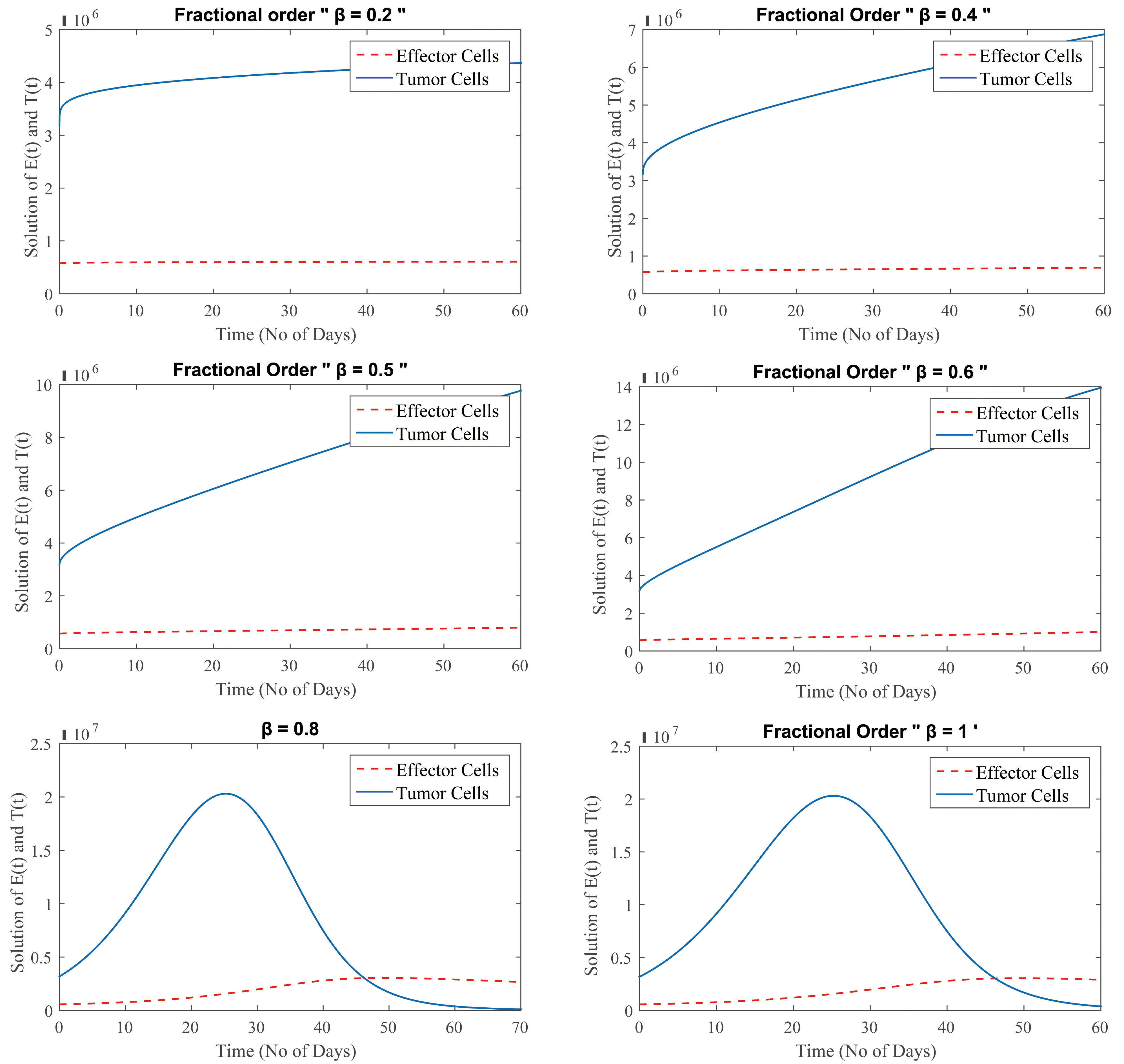
Fig. 1 depicts the proliferation of cancer cells at different fractional orders of $0.2$ , $0.4$ , $0.5$ , $0.6$ , $0.8$ and $1$ following immunotherapy, in which the immune system of the cancer patient is activated. After the immmune system is activated, tumor cells are reduced while effector cells are increased. Tumor cells are weak at the first stage and can be decreased with immunotherapy. Our immune system not only combats cancer cells, but it also eliminates aberrant cells in our bodies. If a patient is diagnosed with cancer that cannot be treated by immunotherapy alone, it is probable that the downstream cells have infiltrated elsewhere, making the effector cells’ job more difficult. Cancer cells begin to decrease as the cells expand.

Fig. 1.

(Model 1) Level of effector and tumor cells at $\beta$ = 0.2, 0.4, 0.5, 0.6, 0.8 and 1.

Moreover, Fig. 1 shows that at $\beta=0.2$ , $0.4$ , $0.5$ , and $0.6$ , the number of tumor cells increases rapidly in 60 days, but the growth of effector cells is slow. At $\beta=0.8$ and $1$ , effector cells increase and tumor cells decrease. The more realistic results are obtained for $\beta=0.8$ than $\beta=1$ as the CT period is 60 to 70 days, approximately.

Generally, the cancer treatment takes longer time when effector cells increase and tumor cells reduce which is depicted in Fig. 1 for $\beta=0.8$ . These results enhance the importance of fractional calculus.

4.4.2 Test Problem 2

Model 2:

In this Test Problem 2, FDEs of cancer treatment with immunotherapy and chemotherapy are considered while taking low-dose chemotherapy and immunotherapy into account. Tumor cells first shrink and then multiply, but as effector cells proliferate, tumor cell development slows again. This process has been shown at different fractional orders.

Fig. 2 shows the graphical representation of Eqn. 2, using immunotherapy and chemotherapy (low concentration) in combination. Fig. 2 depicts that the patient receives combined therapy, the outcome is also favourable, but the immune system is weakened slightly since the chemotherapy kills some effector cells along with the cancer cells. It is also a treatment for early-stage cancer; however, chemotherapy is administered in extremely low dosages. In summary, immunotherapy is used to treat patients with lesser dosages of chemotherapy, resulting in a better prognosis.

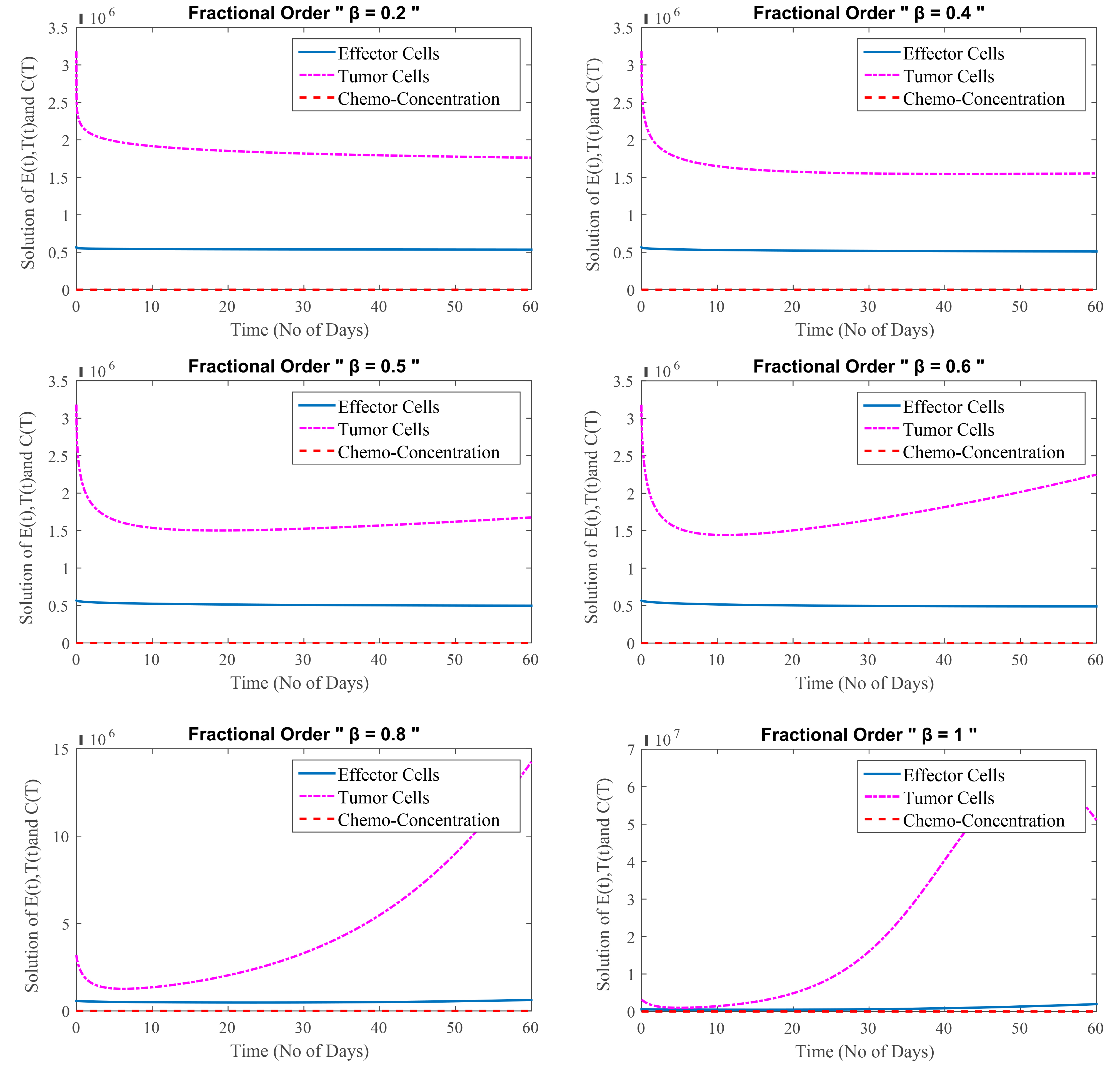
Fig. 2.

(Model 2) Level of effector cells, tumor cells and concentration of chemotherapy at $\beta$ = 0.2, 0.4, 0.5, 0.6, 0.8 and 1.

Fig. 2 shows that at $\beta=0.2,0.4,0.5,$ and $0.6,$ the number of tumor cells decreases rapidly at first, but then slowly increases after a few days of low-dose chemotherapy administered over 60 days, whereas effector cells remain stable. At $\beta=0.8$ the growth of tumor cells begins to increase fastly after a few days. At $\beta=1$ , effector cells increases slowly after 40 days but tumor cells increases rapidly at first, but then decreases in last 10 days.

4.4.3 Test Problem 3

Model 3:

In this test problem, FDEs with inclusion of depression effects are studied. Cancer is being treated intensively because cancer cells have grown extremely powerful. High doses of chemotherapy are combined with immunotherapy, resulting in an increase in effector cells from the immunotherapy and a decrease in tumor cells from the chemotherapy. Chemotherapy, as the treatment progresses, affects the effector cells as well as the tumor cells.

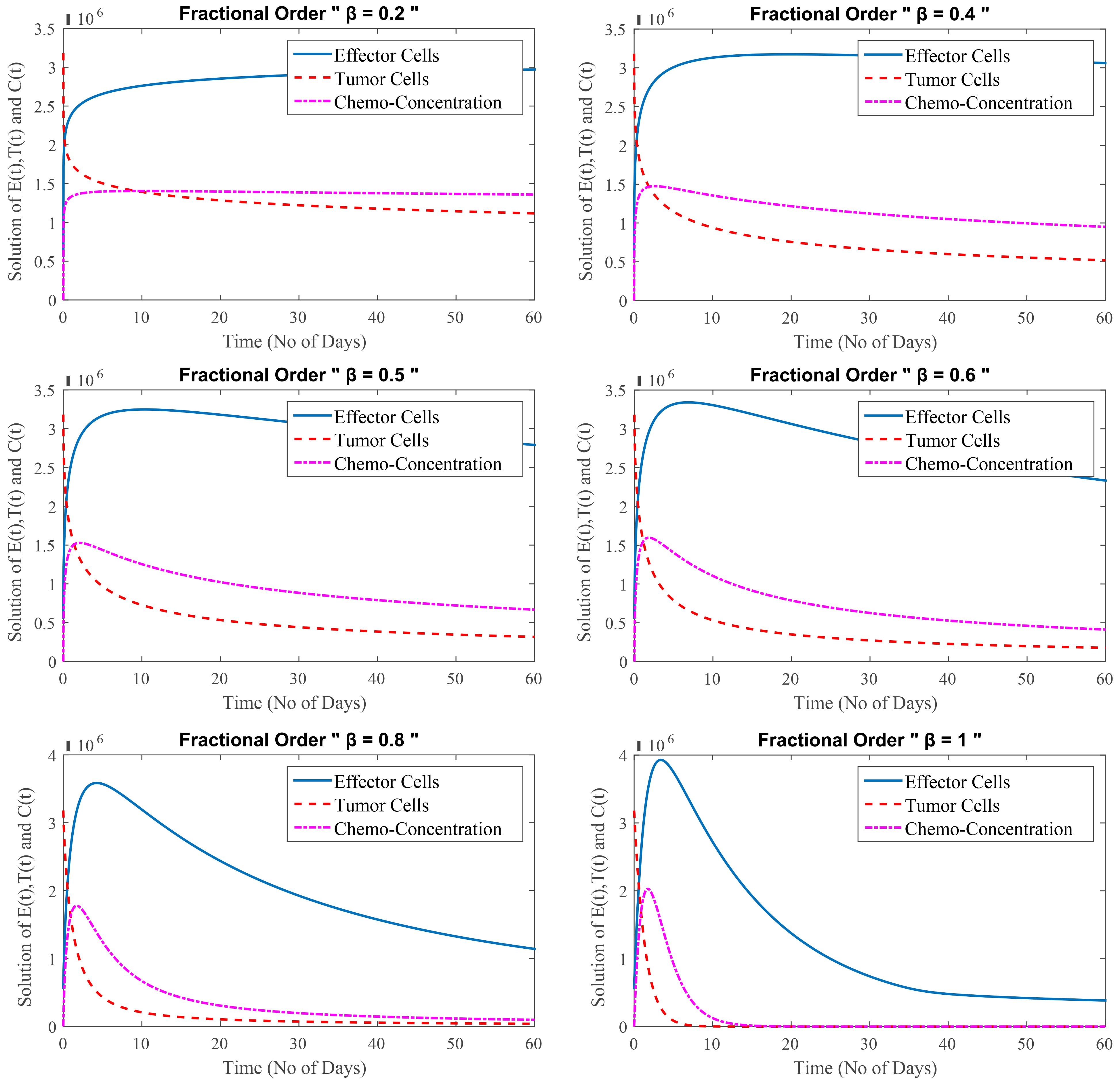
Fig. 3 depicts the relation among effector cells, tumor cells and chemo-concentration for different values of $\beta$ . In Fig. 3, results of the fractional order is presented at $\beta=0.2,0.4,0.5,0.6,0.8$ and $1$ . Here, cancer cells decrease when we use chemotherapy (high concentration) with immunotherapy. After adding chemotherapy, we get some negative effects, which we find that chemo drugs affect tumor or cancer cells as well as some immune or effector cells.

Fig. 3.

(Model 3) Level of effector cells, tumor cells and concentration of chemotherapy at $\beta$ = 0.2, 0.4, 0.5, 0.6, 0.8 and 1.

Fig. 3 shows that at $\beta=0.2,0.4,$ and $0.5$ , the number of effector cells and rate of chemotherapy increase immediately, but the number of tumor cells decrease. Due to the high concentration of chemotherapy, the number of tumor cells decrease quickly, but the number of effector cells initially increase and then decay at $\beta=0.6,0.8,$ and $1$ . Here, the depression term is taken zero.

4.4.4 Test Problem 4

Model 4:

In this test Problem, FDEs of cancer treatment at secondary stage are taken into account. This stage of cancer is known as the secondary stage, or metastasis, and it is extremely dangerous. The effector cells are reduced from the start at this stage, while the tumor cells are suppressed owing to chemotherapy. It is detrimental to patients and can potentially kill them over time because of the weak immune system. Chemotherapy and depression both reduce the number of effector cells. The severe impact of depression with chemotherapy has a negative influence on the immune system, effector cells do not rise with immunotherapy. As a result, the patient is on the verge of death.

Fig. 4 shows that even after a combination of therapies, sadness plays an important role in malignant cells growth. The number of cancerous cells in the first stage is lower than in the later stage. Depression has a greater impact during the secondary stage and has not significant impact during the primary stage. The primary stage of cancer is when the disease first appears. A secondary cancer, on the other hand, can be classified as either a new primary cancer in a different part of the body or a metastasis of the original primary cancer to another part of the body.

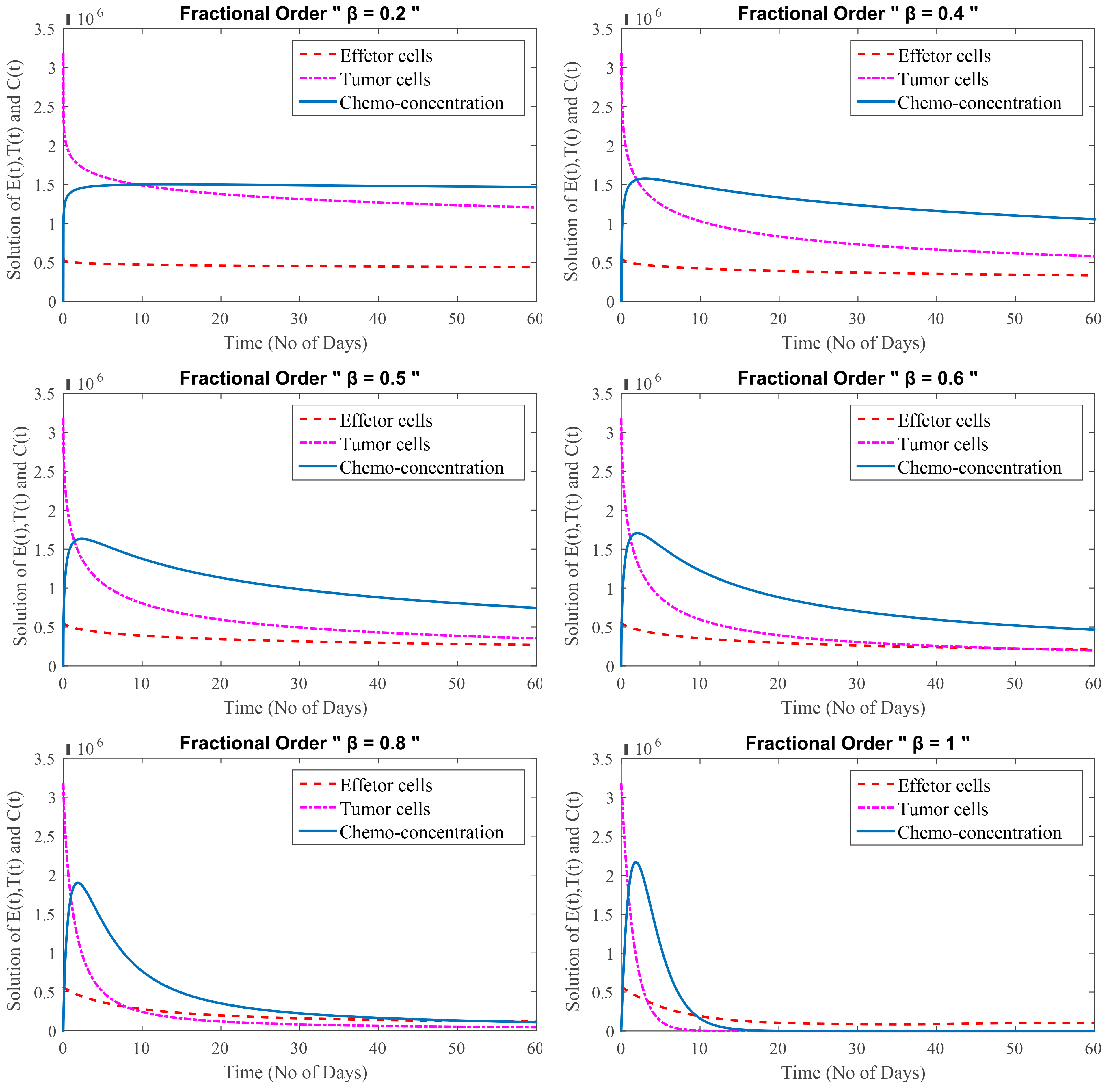
Fig. 4.

(Model 4) Level of effector cells, tumor cells and concentration of chemotherapy with minimum depression effect at $\beta$ = 0.2, 0.4, 0.5, 0.6, 0.8 and 1.

Fig. 4 shows that at $\beta=0.2$ , the number of tumor cells decrease quickly at the start and then decrease slowly and gradually. The rate of chemotherapy increases at first, but effector cells do not grow. The number of tumor cells decreases quickly at $\beta=0.4,0.5,$ and $0.6,$ and the chemo-concentration increases and then decreases. Effector cells are also deteriorating, which is a bad news for the patient. In Fig. 4, the rate of chemotherapy increases rapidly and then decays. Due to the high concentration of chemotherapy, the number of tumor cells decrease very quickly, and effector cells are also decaying at $\beta=0.8$ and $1$ .

Cancer survival rates, or survival statistics, indicate the percentage of people who survive a specific type of cancer over a given time period. Statistics on cancer frequently use a five-year overall survival rate. The cancer survival rate is affected by a variety of factors, including the type of cancer, the time since diagnosis, and the patient’s age. For example, typically, survival rates are expressed in percentages. For instance, 77 percent of bladder cancer patients survive for at least five years overall. In other words, 77 out of every 100 bladder cancer patients are still alive five years after their diagnosis. In contrast, 23 out of every 100 people who are diagnosed with bladder cancer pass away within five years.

On the basis of these results, we conclude that the fractional models gives a better approximation for $\beta$ = 0.7 as compared to $\beta$ = 1. The reasonable range of fractional order is between $\beta$ = $0.6$ and $\beta$ = $0.9$ .

Here, we are discussing the secondary stage, during which the patient is unable to handle such strong medication for an extended period of time since his immune system has already been weakened significantly as a result of cancer cells and depression. This estimate states that the patient has an average remaining life expectancy of five years, or 1825 days, at this point. Here, $\beta$ is chosen $0.7$ , which maintains the balance of all three factors and prolongs the life of the patient, even if patient is elderly or had a late diagnosis.

4.5 High Depression Effects in Secondary Stage

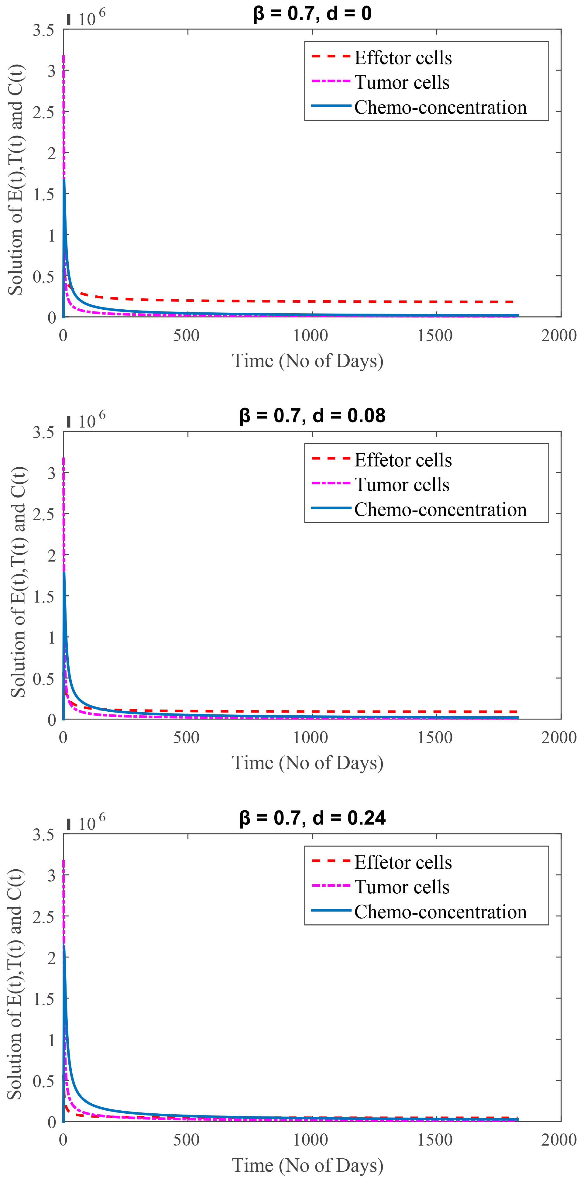
One of the most significant concern among cancer patients in the secondary stage is depression. Fig. 5 displays the depression effects on patient’s health considering $d=0,d=0.08$ , and $d=0.24$ . According to medical studies, the number of cancer patients who experience depression ranges from 8 percent to 24 percent, and we are currently observing the 24 percent depression effect in the secondary stage of model (c.f. Eqn. 4).

Fig. 5.

(Model 4) Time period of 5 years.

The graphical representation clearly shows how high depression affects immune cells, causing them to weaken. It means cancer patients not only need medical treatment but also your care and support to fight against cancer.

4.6 Effects of Some More Parameters

This section focuses on the effects of several important parameters. In the simulations, we change one parameter while fixing the values of the other parameters. Here, $\beta=0.7$ is taken into account.

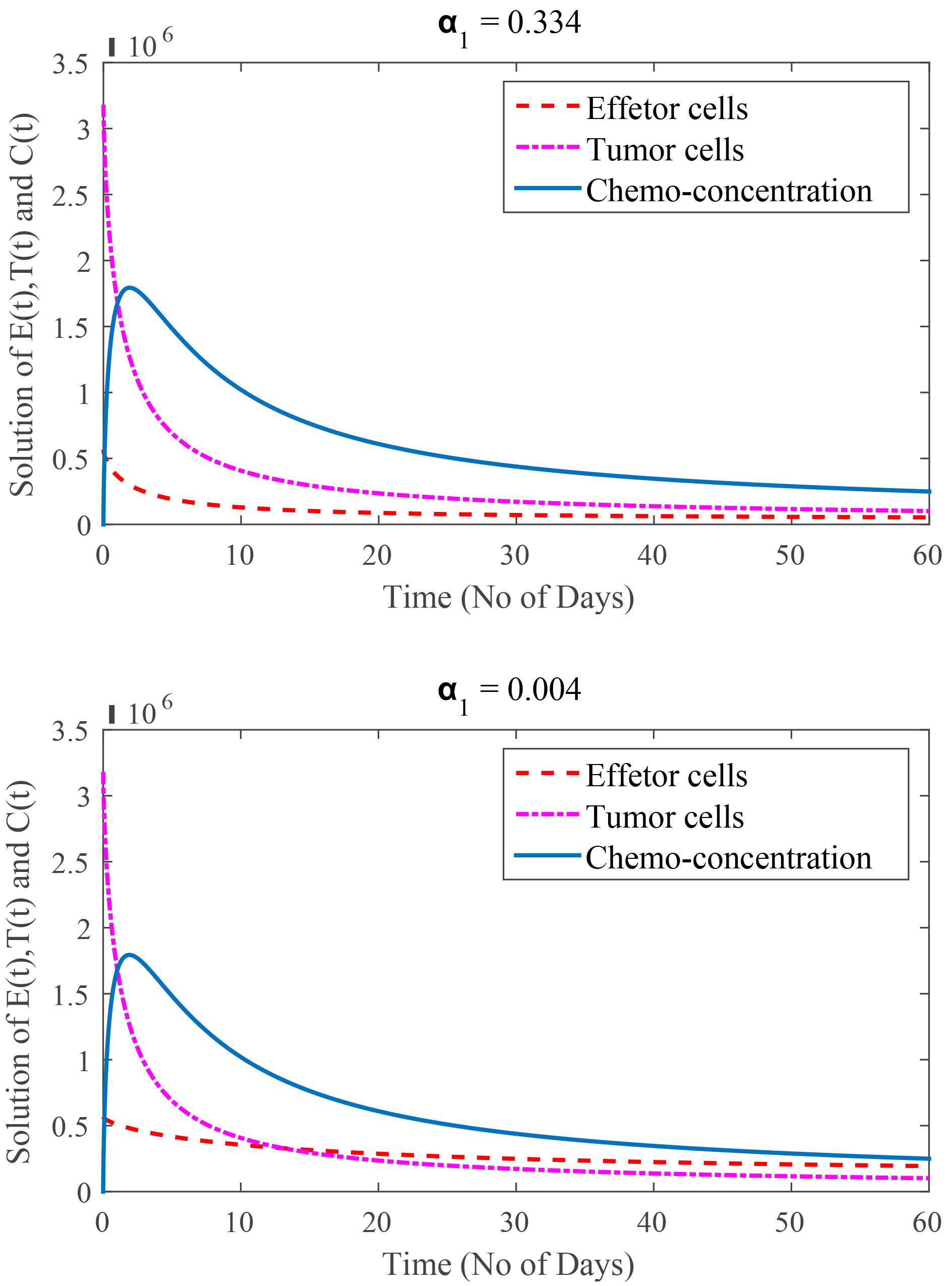
In Fig. 6, the value of $\alpha_{1}$ is varied, while all other parameter values are kept fixed. The solution is found for two different values of the effect of chemotherapy on the fractional immune cell rate, namely $\alpha_{1}$ $(0.334,0.004)$ . It is found that as the quantitative value of the killing rate of chemotherapy on immune cells increases, the number of effector cells decreases. The decrease in the value of the killing rate from chemotherapy to immune cells shows effector cells survive more.

Fig. 6.

(Model 4) Rate of immune cells kill by chemotherapy are $\alpha_{1}$ = 0.334 and 0.004, at $\beta$ = 0.7.

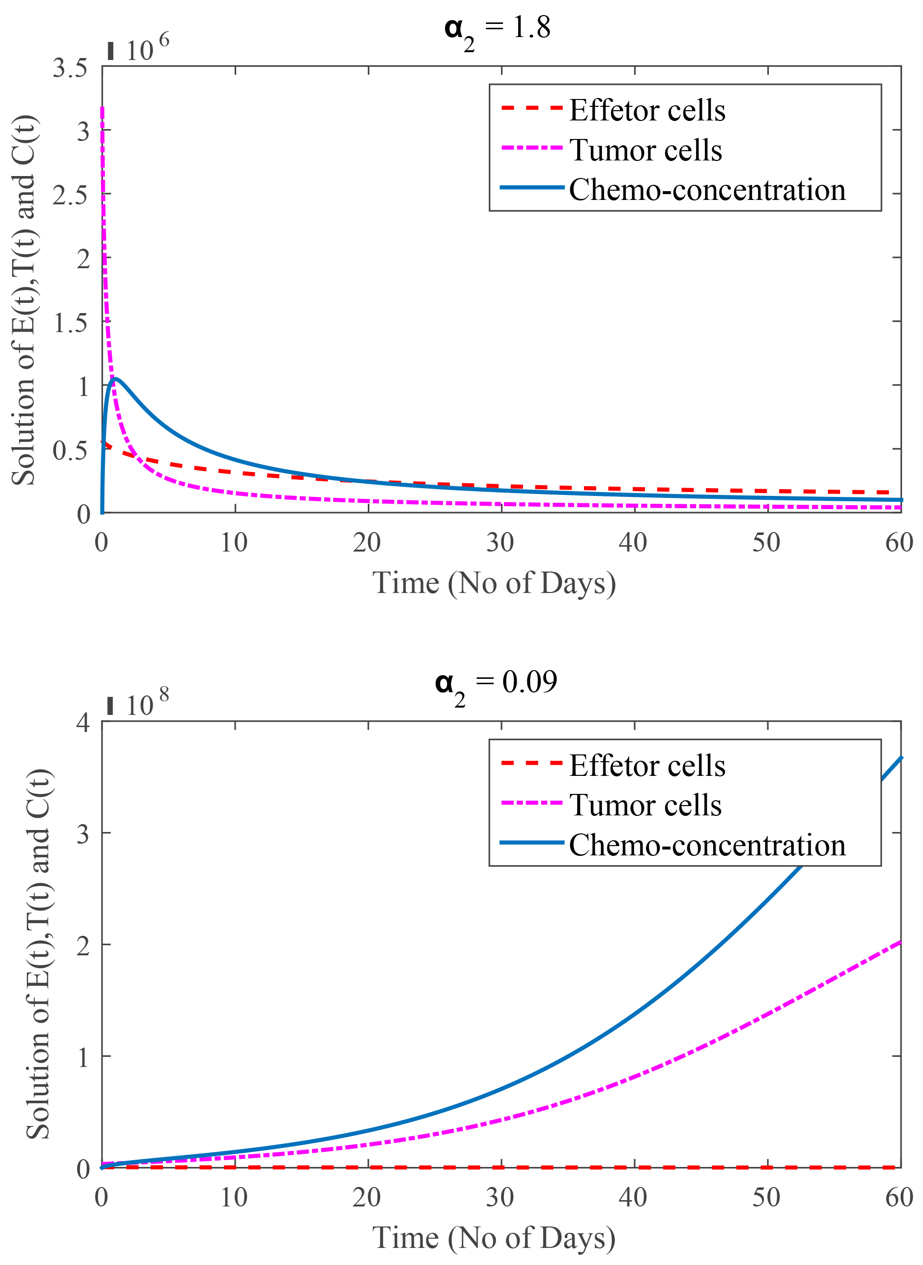
In Fig. 7, the value of $\alpha_{2}$ is varied, while all other parameter values are kept fixed. The solution is found for two different chemotherapy doses that kill fractional tumor cells at the same rate, namely $\alpha_{2}$ $(1.8,0.09)$ . It is found that as the quantitative value of the killing rate of chemotherapy on tumor cells increases, the number of tumor cells decreases. The decrease in the value of the killing rate from chemotherapy for tumor cells shows effector cells are dead and tumor cells are increasing.

Fig. 7.

(Model 4) Rate of tumor cells kill by chemotherapy are $\alpha_{2}$ = 1.8 and 0.09, at fractional order 0.7.

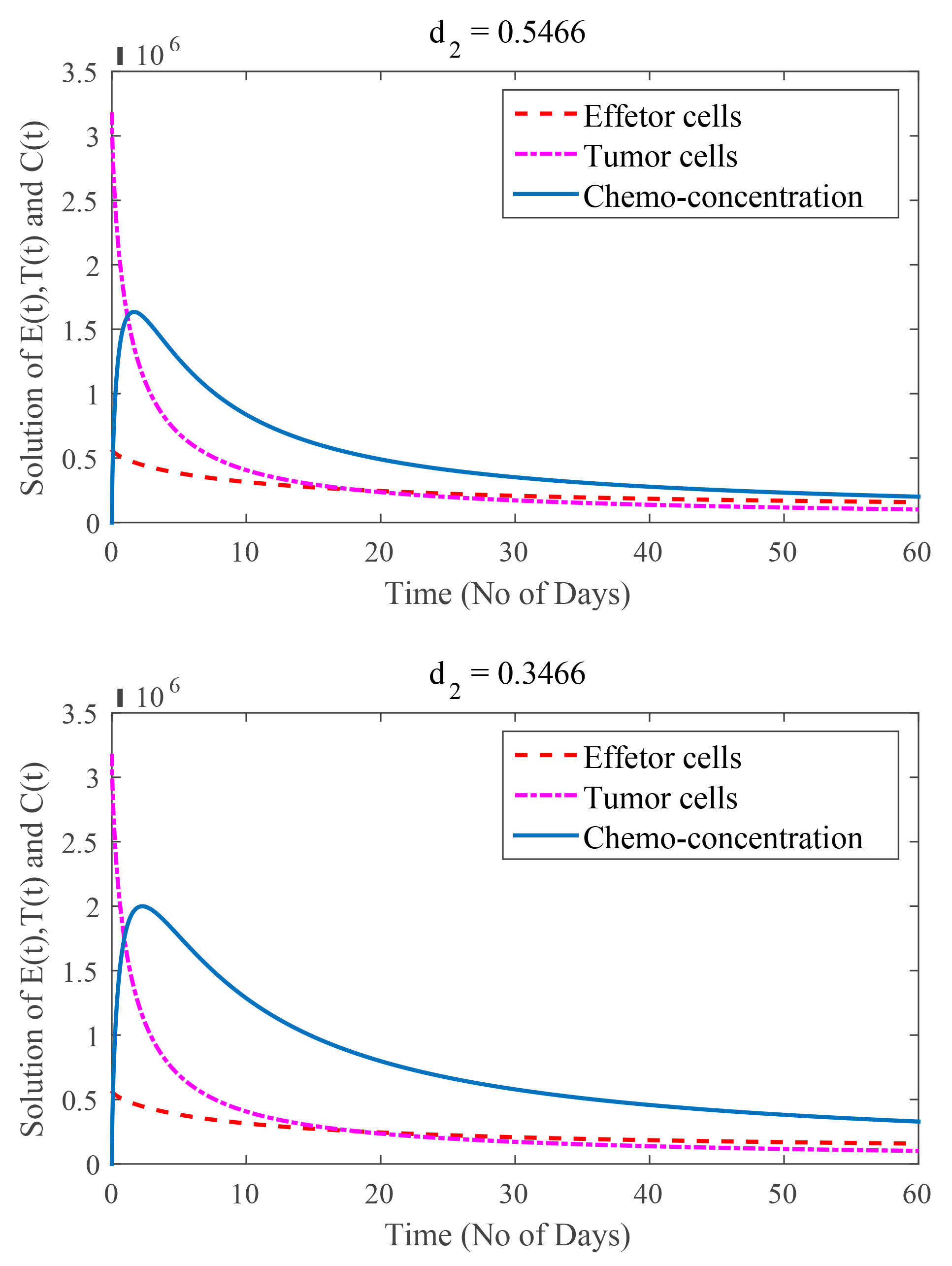
In Fig. 8, the value of $d_{2}$ is varied while the values of all other parameters remain constant. The solution is found for two different chemotherapy degradation rate effects, namely $d_{2}$ $(0.5466,0.3466)$ . It is found that as the quantitative value of the decaying rate of chemotherapy increases, the number of effector and tumor cells decreases at the same rate, but the concentration of chemotherapy begins to decrease quickly. The decrease in the value of the decaying rate of chemotherapy shows a late decline in the chemotherapy concentration. The parametric study verifies the correctness of the model formulation.

Fig. 8.

(Model 4) Rate of chemotherapy drug decay are $d_{2}$ = 0.5466 and 0.3466, at $\beta$ = 0.7.

4.7 Curve Fitting Procedure

The act of creating the mathematical function or curve that best fits a set of data points, perhaps subject to limitations, is known as “curve fitting”. A “smooth” function that roughly matches the data is created during curve fitting, as opposed to interpolation, which requires a perfect fit to the data. Discrete data points are connected using interpolation in order to provide realistic estimates of the data points between the given ones. Finding the curve that would best represent the trend of a given collection of data is known as “curve fitting”.

The curve fitting is applied for Model 4. The procedure is repeated for tumor cells, chemo-concentration (chemotherapy), and effector Cells, graphically presented in Fig. 9 and Fig. 10 Tables 2,3 display the information. It has been proposed to have a bi-exponential model as presented in Eqn. 44 by observing the nature of the data.

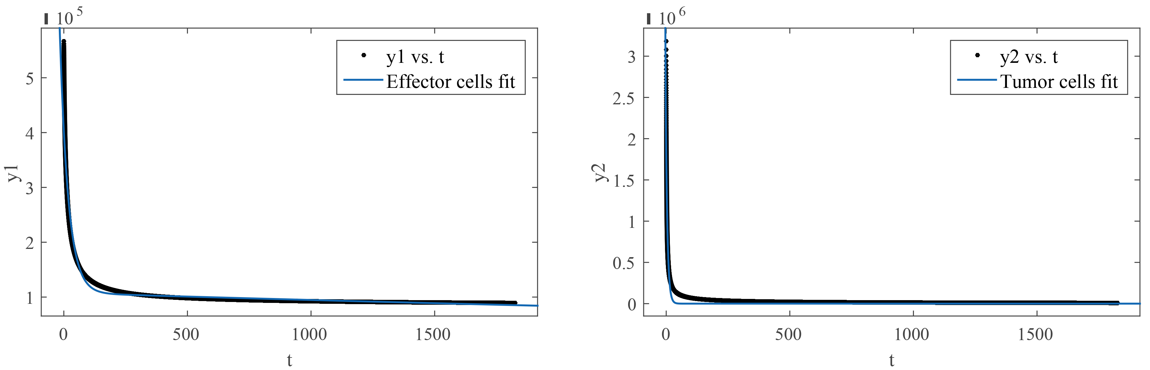
Fig. 9.

(Model 4) Curve fitting on effector cells and tumor cells.

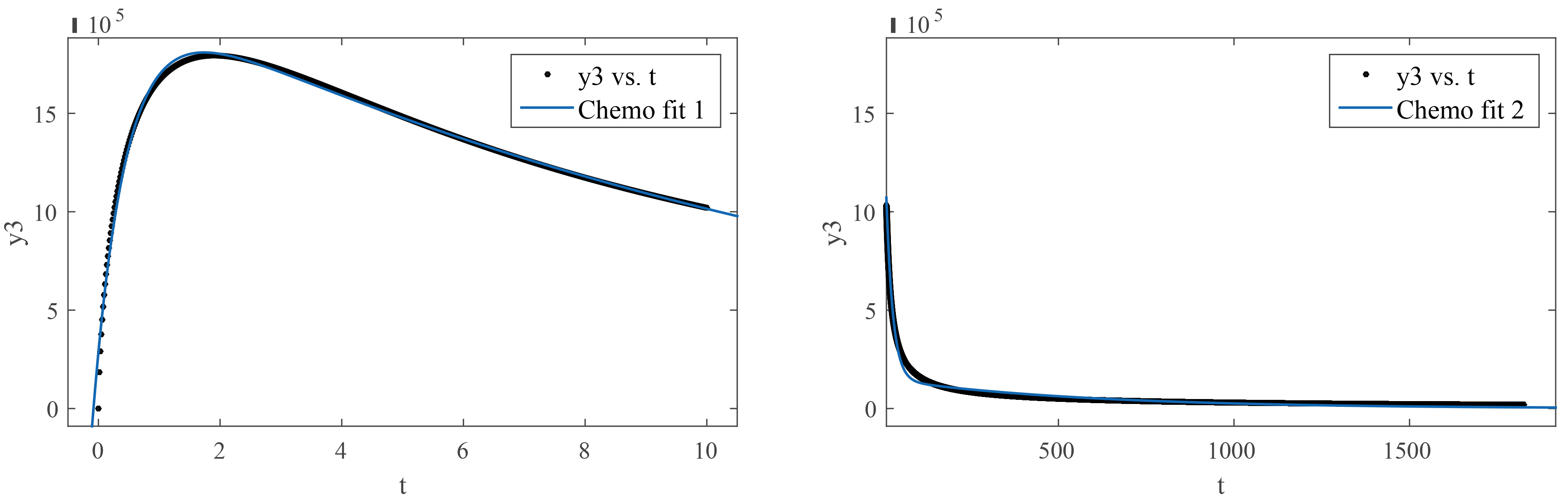
Fig. 10.

(Model 4) Curve fitting of chemo-concentration at time 0 to 10 and 10 to 1825 days.

Table 2.Estimation of coefficients.

Name of variables	a ${}_{\text{i}}$	b ${}_{\text{j}}$	c ${}_{\text{k}}$	d ${}_{\text{l}}$
Effector cells	$3.187e+05$	$-0.035$	$1.098e+05$	$-0.0001444$
Tumor cells	$2.11e+06$	$-0.2776$	$1.904e+05$	$-0.006999$
Chemo-concentration (0–10)	$2.149e+06$	$-0.07499$	$-1.864e+06$	$-1.835$
Chemo-concentration (10–1825)	$1.558e+06$	$-0.05334$	$1.506e+05$	$-0.001759$

Table 3.Estimation of constants used in Eqn. 44 based on the least square error method, along with goodness of fit parameters.

Name of variables	SSE	R-square	Adjusted R-square	RMSE
Effector cells	$4.089e+12$	0.9645	0.9645	5917
Tumor cells	$3.659e+13$	0.9544	0.9544	$1.77e+04$
Chemo-concentration (0–10)	$2.575e+11$	0.995	0.9949	$2.011e+04$
Chemo-concentration (10–1825)	$6.308e+13$	0.9685	0.9685	$2.324e+04$

Abbreviations: SSE, Sum of Squares; RMSE, Root mean square error.

(44) $\begin{gathered}\displaystyle f(x)=a_{i}e^{b_{j}x}+c_{k}e^{d_{l}x},\quad i,j,k% ,1=1,2,3,4\end{gathered}$

where $a_{i},b_{j},c_{k},d_{l}$ are coefficients and presented in Table 2.

Exponentials are often used when the rate of change of a quantity is proportional to the initial amount of the quantity. If the coefficient associated with $b_{j}$ and/or $d_{l}$ is negative, $f(x)$ represents exponential decay. If the coefficient is positive, $y$ represents exponential growth. For example, a single radioactive decay mode of a nuclide is described by a one-term exponential. a is interpreted as the initial number of nuclei, $b_{j}$ is the decay constant, $x$ is time, and $y$ is the number of remaining nuclei after a specific amount of time passes. If two decay modes exist, then you must use the two-term exponential model. For the second decay mode, you add another exponential term to the model. Examples of exponential growth include contagious diseases for which a cure is unavailable, and biological populations whose growth is uninhibited by predation, environmental factors, and so on.

The careful selection of a mathematical function able to accurately represent the data was based on various parameters of “goodness of fit” like SSE, R-squared values, adjusted R-squared values, and root mean square error (RMSE). Other functions are likely to present poor values for goodness of fit. We have bi exponential model of Eqn. 44 for representation of all experiments. It can be observed that “ $b_{j}$ ” and “ $d_{l}$ ” are coefficients representing the decay constant in the bi-exponential model. The values of “ $b$ ” are more important and play a vital role in deciding the decay factor.

Eqn. 44 is very useful for medical practitioners to treat the cancer patients. In Eqn. 44, $x$ is used in place of time (number of days). One can see the results of three classes (effector cells, tumor cells, and chemo-concentration) by putting the value of any time in Eqn. 44 considering Table 2. These derived results are beneficial for medical practitioners to choose the chemo-concentration and their effects on tumor cells. Furthermore, medical practitioners can validate the obtained results in real scenarios. This study will open the new directions to treat cancer.

5. Conclusions

The purpose of this work was to study a fractional models for cancer treatment with mixed therapies. In this work, different fractional models was theoretically studied. The model contains system of FDEs which incorporate the effector cells, tumor cells and rate of chemotherapy. Stability analysis was done using Lyapunov function. Moreover, positivity and boundedness of the solution was proved. Furthermore parametric study and curve fitting procedure was also discussed. The results are presented for four different models of primary and secondary stage for cancer treatment.

The results indicate that, before treating a cancer patient, it is important to know the stage of the disease. We were able to control tumor cells during the primary stage, but it was more difficult to control cancer cells during the secondary stage due to a reduction in immune cells caused by chemotherapy and depression. We found that the first stage of cancer or tumor growth is slower than the secondary stage. Effect of some positive parameters are weakens because effect of depression is higher than secondary stage.

The loss of immune cells is a key factor in tumor progression. In this paper, we provided the findings of a mathematical model that shows sadness decreases immune cell counts while increases tumor cell counts. As the patient is unaware that he has cancer in its early stages, depression has little impact on either immune cells or tumor cells. As soon as he learns, the patient is affected by depression. As the effects of depression worsen, the patient’s immunity declines, which increases the number of tumor cells. The impact of chemotherapy is very low, nearly inert, and the patient might die from depression as the effect of depression develops and the tumor cells grow significantly. The fractional model of the secondary stage gave a better approximation for $\beta=0.7$ as compared to $\beta=1$ . For all fractional models the reasonable range of fractional order is between $\beta=0.6$ and $\beta=0.9$ . The function obtained from curve fitting may help doctors for finding the optimal dosage of chemo-concentration and its effects.

Future researches may explore parameter estimation, the inclusion of different doses in chemotherapy which may not weak the immune system. This study is an effort to provide more profound insights into various aspects of cancer disease and its treatment.

Availability of Data and Materials

Datasets used and/or analyzed for this study are available from the corresponding author upon appropriate request.

Author Contributions

SJ: Conceptualization, investigation, methodology, analysis, and writing–original draft, review, supervision and project administration. ZA: Investigation, analysis, validation and writing–original draft and review. DB: Validation, formal analysis, supervision, and project administration. All authors have contributed to the manuscript and approved the submitted version. All authors have read and agreed to the published version of the manuscript. All authors have participated sufficiently in the work and agreed to be accountable for all aspects of the work.

Ethics Approval and Consent to Participate

Not applicable.

Acknowledgment

Not applicable.

Funding

This research received no external funding.

Conflict of Interest

The authors declare no conflict of interest. DB is serving as one of the Guest editors of this journal. We declare that DB had no involvement in the peer review of this article and has no access to information regarding its peer review. Full responsibility for the editorial process for this article was delegated to SL.

References

[1]

AL-Azzawi SN, Shihab FA, Al-Sayyid MM. Solution of modified Kuznetsov model with mixed therapy. Global Journal of Pure and Applied Mathematics. 2017; 13: 6269–6288.

| Google Scholar

[2]

Mamat M, Subiyanto KA, Kartono A. Mathematical model of cancer treatments using immunotherapy, chemotherapy and biochemotherapy. Applied Mathematical Sciences. 2013; 7: 247–261.

| Google Scholar

[3]

Liu Z, Yang C. A mathematical model of cancer treatment by radiotherapy. Computational and Mathematical Methods in Medicine. 2014; 2014: 172923.

| Google Scholar

[4]

Mishel MH, Hostetter T, King B, Graham V. Predictors of psychosocial adjustment in patients newly diagnosed with gynecological cancer. Cancer Nursing. 1984; 7: 291–299.

| Google Scholar

[5]

Linden W, Vodermaier A, Mackenzie R, Greig D. Anxiety and depression after cancer diagnosis: prevalence rates by cancer type, gender, and age. Journal of Affective Disorders. 2012; 141: 343–351.

| Google Scholar

[6]

de Pillis LG, Gu W, Radunskaya AE. Mixed immunotherapy and chemotherapy of tumors: modeling, applications and biological interpretations. Journal of Theoretical Biology. 2006; 238: 841–862.

| Google Scholar

[7]

Kim Y, Lee D, Lee J, Lee S, Lawler S. Role of tumor-associated neutrophils in regulation of tumor growth in lung cancer development: A mathematical model. PLoS ONE. 2019; 14: e0211041.

| Google Scholar

[8]

Bashkirtseva I, Ryashko L, Duarte J, Seoane JM, Sanjuan MA. The role of noise in the tumor dynamics under chemotherapy treatment. The European Physical Journal Plus. 2021; 136: 1–13.

| Google Scholar

[9]

Ahmad S, Javeed S, Ahmad H, Khushi J, Elagan SK, Khames A. Analysis and numerical solution of novel fractional model for dengue. Results in Physics. 2021; 28: 104669.

| Google Scholar

[10]

Zafar ZUA, Hussain MT, Inc M, Baleanu D, Almohsen B, Oke AS, et al. Fractional-order dynamics of human papillomavirus. Results in Physics. 2022; 34: 105281.

| Google Scholar

[11]

Javeed S, Anjum S, Alimgeer KS, Atif M, Khan MS, Farooq WA, et al. A novel mathematical model for COVID-19 with remedial strategies. Results in Physics. 2021; 27: 104248.

| Google Scholar

[12]

Javeed S, Qamar S, Ashraf W, Warnecke G, Seidel-Morgenstern A. Analysis and numerical investigation of two dynamic models for liquid chromatography. Chemical Engineering Science. 2013; 90: 17–31.

| Google Scholar

[13]

d’Onofrio A, Ledzewicz U, Maurer H, Schättler H. On optimal delivery of combination therapy for tumors. Mathematical Biosciences. 2009; 222: 13–26.

| Google Scholar

[14]

Kermack WO, McKendrick AG. A contribution to the mathematical theory of epidemics. Proceedings of the royal society of london. Series A, Containing papers of a mathematical and physical character. 1927; 115: 700–721.

| Google Scholar

[15]

Kermack WO, McKendrick AG. Contributions to the mathematical theory of epidemics: V. Analysis of experimental epidemics of mouse-typhoid; a bacterial disease conferring incomplete immunity. The Journal of Hygiene. 1939; 39: 271–288.

| Google Scholar

[16]

Sweilam NH, Al-Mekhlafi SM, Albalawi AO, Machado JT. Optimal control of variable-order fractional model for delay cancer treatments. Applied Mathematical Modelling. 2021; 89: 1557–1574.

| Google Scholar

[17]

Sowndarrajan PT, Manimaran J, Debbouche A, Shangerganesh L. Distributed optimal control of a tumor growth treatment model with cross-diffusion effect. The European Physical Journal Plus. 2019; 134: 463.

| Google Scholar

[18]

Ozdemir N, Ucar E. Investigating of an immune system-cancer mathematical model with Mittag-Leffler kernel. AIMS Math. 2020; 5: 1519–1531.

| Google Scholar

[19]

de Pillis LG, Radunskaya AE, Wiseman CL. A validated mathematical model of cell-mediated immune response to tumor growth. Cancer Research. 2005; 65: 7950–7958.

| Google Scholar

[20]

Mufudza C, Sorofa W, Chiyaka ET. Assessing the effects of estrogen on the dynamics of breast cancer. Computational and Mathematical Methods in Medicine. 2012; 2012: 473572.

| Google Scholar

[21]

Abernathy K, Abernathy Z, Baxter A, Stevens M. Global Dynamics of a Breast Cancer Competition Model. Differential Equations and Dynamical Systems. 2020; 28: 791–805.

| Google Scholar

[22]

Jarrett AM, Shah A, Bloom MJ, McKenna MT, Hormuth DA, 2nd, Yankeelov TE, et al. Experimentally-driven mathematical modeling to improve combination targeted and cytotoxic therapy for HER2+ breast cancer. Scientific Reports. 2019; 9: 12830.

| Google Scholar

[23]

Liu Z, Zhong S, Yin C, Chen W. Permanence, extinction and periodic solutions in a mathematical model of cell populations affected by periodic radiation. Applied Mathematics Letters. 2011; 24: 1745–1750.

| Google Scholar

[24]

Freedman HI, Belostotski G. Perturbed models for cancer treatment by radiotherapy. Differential Equations and Dynamical Systems. 2009; 17: 115–133.

| Google Scholar

[25]

Eskandari Z, Avazzadeh Z, Khoshsiar Ghaziani R, Li B. Dynamics and bifurcations of a discrete‐time Lotka–Volterra model using nonstandard finite difference discretization method. Mathematical Methods in the Applied Sciences. 2022.

| Google Scholar

[26]

Li B, Liang H, Shi L, He Q. Complex dynamics of Kopel model with nonsymmetric response between oligopolists. Chaos, Solitons & Fractals. 2022; 156: 111860.

| Google Scholar

[27]

Li B, Liang H, He Q. Multiple and generic bifurcation analysis of a discrete Hindmarsh-Rose model. Chaos, Solitons & Fractals. 2021; 146: 110856.

| Google Scholar

[28]

Li B, Zhang Y, Li X, Eskandari Z, He Q. Bifurcation analysis and complex dynamics of a Kopel triopoly model. Journal of Computational and Applied Mathematics. 2023; 426: 115089.

| Google Scholar

[29]

Zeb A, Chohan MI, Zaman G. The homotopy analysis method for approximating of giving up smoking model in fractional order. Applied Mathematics. 2012; 3: 914–919.

| Google Scholar

[30]

Liu X, Arfan M, Ur Rahman M, Fatima B. Analysis of SIQR type mathematical model under Atangana-Baleanu fractional differential operator. Computer Methods in Biomechanics and Biomedical Engineering. 2023; 26: 98–112.

| Google Scholar

[31]

Zafar Z, Zaib S, Tanveer C, Tunc C, Javeed S. Analysis and numerical simulation of tuberculosis model using different fractional derivatives, Chaos, Soliton & Fractals. 2022; 160: 112202.

| Google Scholar

[32]

Podlubny I. Fractional differential equations. Mathematics in science and engineering. 1999; 198: 41–119.

| Google Scholar

[33]

El Maroufy H, Lahrouz A, Leach PGL. Qualitative behaviour of a model of an SIRS epidemic: stability and permanence. Applied Mathematics & Information Sciences. 2011; 5: 220–238.

| Google Scholar

Publisher’s Note: IMR Press stays neutral with regard to jurisdictional claims in published maps and institutional affiliations.

Fig. 1.

(Model 1) Level of effector and tumor cells at $\beta$ = 0.2, 0.4, 0.5, 0.6, 0.8 and 1.

1 of 10

Front. Biosci. (Landmark Ed) Print ISSN 2768-6701 Electronic ISSN 2768-6698