
Academic Editor: Alexandros G. Georgakilas
Background: In biomedical and epidemiological studies, gene-environment (G-E) interactions play an important role in the etiology and progression of many complex diseases. In ultra-high-dimensional survival genomic data, two common approaches (marginal and joint models) are proposed to determine important interaction biomarkers. Most existing methods for detecting G-E interactions (marginal Cox model and marginal accelerated failure time model) are limited by a lack of robustness to contamination/outliers in response outcome and prediction biomarkers. In particular, right-censored survival outcomes and ultra-high-dimensional feature space make relevant feature screening even more challenging. Methods: In this paper, we utilize the non-parametric Kendall’s partial correlation method to obtain pure correlation to determine the importance of G-E interactions concerning clinical survival data under a marginal modeling framework. Results: A series of simulated scenarios are conducted to compare the performance of our proposed method (Kendall’s partial correlation) with some commonly used methods (marginal Cox’s model, marginal accelerated failure time model, and censoring quantile partial correlation approach). In real data applications, we utilize Kendall’s partial correlation method to identify G-E interactions related to the clinical survival results of patients with esophageal, pancreatic, and lung carcinomas using The Cancer Genome Atlas clinical survival genetic data, and further establish survival prediction models. Conclusions: Overall, both simulation with medium censoring level and real data studies show that our method performs well and outperforms existing methods in the selection, estimation, and prediction accuracy of main and interacting biomarkers. These applications reveal the advantages of the non-parametric Kendall’s partial correlation approach over alternative semi-parametric marginal modeling methods. We also identified the cancer-related G-E interactions biomarkers and reported the corresponding coefficients with p-values.
In order to understand, model, and treat complex diseases such as diabetes, cancer and so on, gene-environment (G-E) interaction has been shown to be a significant role beyond the main genetic (G) or environmental (E) effects [1, 2]. G-E interaction has important implications for the etiology and progression of many complex diseases. For example, Batchelor, et al. [3] demonstrated that the interaction between gene TP53 and environmental factor age to affected the prognosis of glioblastoma. To this end, we would like to identify significant interaction biomarkers that are associated with clinical survival outcomes, which is a crucial task for establishing survival prediction models.
According to Zhou, et al. [4], several statistical methods have been developed to identify significant G-E interactions biomarkers. In high-dimensional genetic data, two general approaches are proposed to identify important interacting biomarkers and estimate their corresponding effects. One performs a marginal analysis, considering only one gene at a time; the other performs a joint analysis and considers all genes in a single model.
In the framework of marginal analysis, for each gene, to fit a model consisting of the single gene itself, consider a few E factors, and its interaction with E factors. The conceptual marginal model is “Outcome ~ Es + G + G * (Es)”, where the response outcome variable can be continuous phenotypes, categorical disease status or patients’ survival time, Es represents a set of environmental factors include environmental exposures as well as demographic, clinical and socioeconomic variables, and G*(Es) represents the interaction between the G factor and all E factors. The significant G-E interaction can be identified based on the correspondence of the marginal p-value. Since the marginal model is low-dimensional, the main advantage of the marginal model is its computational stability and conceptual simplicity; accordingly, marginal programs are still popular in the fields of bioinformatics and biomedicine. In particular, marginal popular models include the accelerated failure time (AFT) model and Cox’s model.
However, a common limitation of traditional marginal analysis methods is their lack of robustness. In actual genetic studies, Xu, et al. [5] noted that long-tailed distributions and contamination in prognostic response outcomes and predictor biomarkers are not uncommon. In addition, human input errors can also lead to long-tailed distributions and contamination. The long-tailed distribution of the survival time means the survival data has a higher rate of censoring. Due to the censoring rate being higher, the proportion of missing survival time is higher. Therefore, the long-tailed distribution of the survival time can lead to the poor performance of the statistical methods.
In Fig. 1, we analyze The Cancer Genome Atlas (TCGA) clinical survival data for esophageal carcinoma (ESCA), pancreatic adenocarcinoma (PAAD) and head and lung adenocarcinoma (LUAD) to show the long-tailed distribution phenomenon. In the top three panels of Fig. 1, the dashed line is the sample mean of logarithm of survival time (months) minus three times standard deviations of survival time (months), which is the 99.73% confidence interval, but we observe that there are still some cancer patients outside the 99.73% confidence interval. Looking at the bottom three panels, the dashed line is the density of fitted normal distribution for logarithm of survival time (months) and the solid line is the empirical density function for logarithm of survival time (months), so it can be seen that the empirical distribution of the actual survival data of cancer patients is different from the fitted normal distribution. And, we also performed an Anderson-Darling test for normality, with the test statistic focusing on a good fit with more emphasis on the tails. The corresponding p-values for ESCA, PAAD, and LUAD are 6e-04, 3e-03, and 3.5e-05, respectively. We have strong evidence to claim that the logarithm of survival times for TCGA data does not follow a normal distribution.
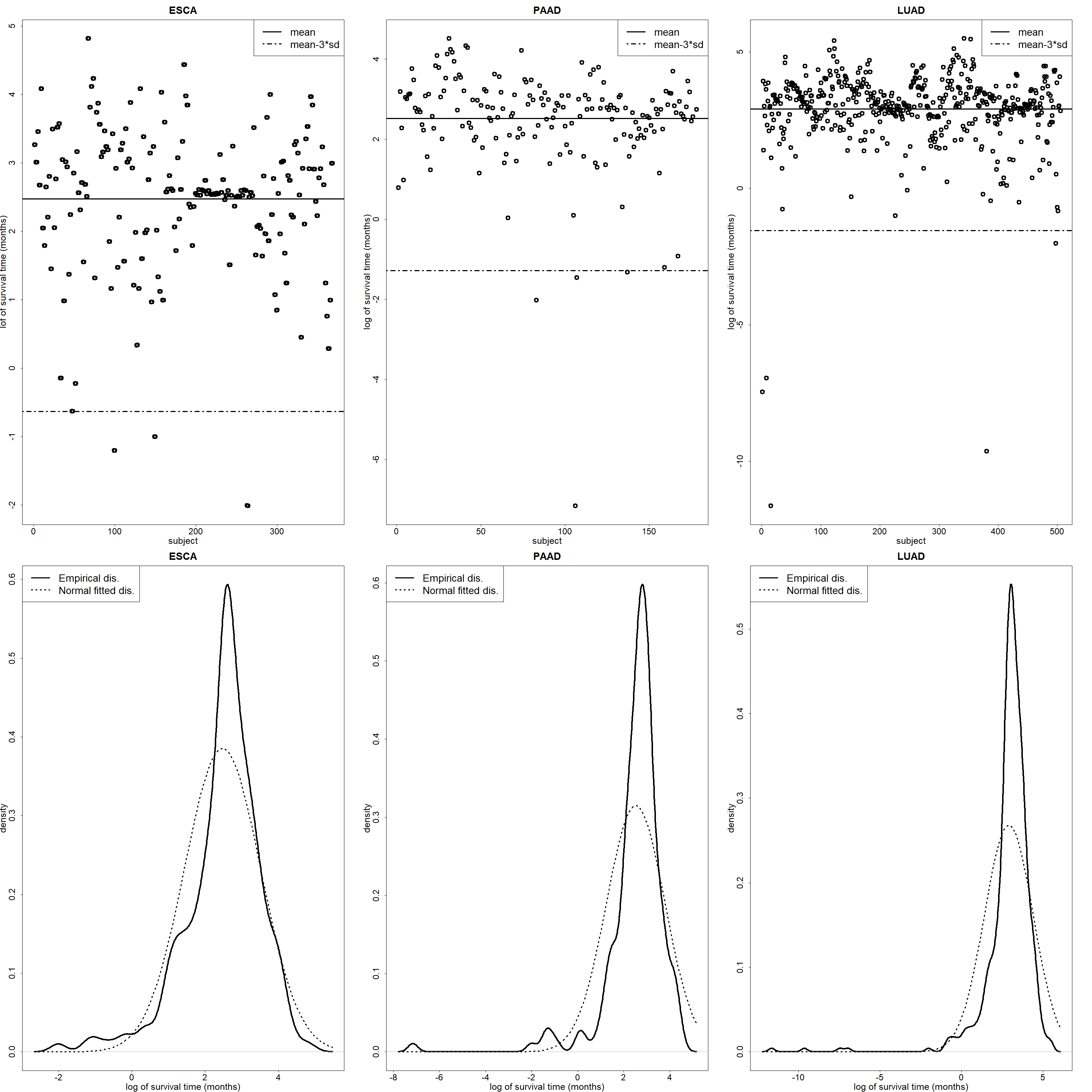 Fig. 1.
The scatter plot and long-tailed distribution of clinical survival time data for the TCGA ESCA, PAAD, and LUAD.
From these two viewpoints, it can be inferred that the survival data is contaminated. Moreover, censored survival outcomes make the relevant feature screening difficult, so several robust methods are proposed to overcome the problem based on the marginal analysis framework [5, 6, 7].
Xu, et al. [5] developed the censored quantile partial correlation approach (CQPCorr) to identify G-E interactions. The CQPCorr approach is built on the quantile regression technique, utilizes weights to accommodate censoring, and adopts a partial correlation to obtain pure correlation for response and interaction biomarker by controlling the main genetic and environmental effects. Shi, et al. [6] developed a robust rank-based estimation approach for the identification of G-E interaction, which is less sensitive to model specification, but computation-demanding.
Furthermore, Wang and Chen [8] proposed an inverse probability-of-censoring weighted (IPCW) Kendall’s tau statistic to measure the association of a right-censored survival trait with biomarkers, and the associated Kendall’s partial correlation reflect the relationship of the survival trait with second-order variables containing quadratic and two-way interactions conditional on the main effects. In simulation studies and real data applications, they demonstrate that the newly proposed method can provide substantially higher accuracy of gene-gene interaction selection hence leading to more accurate survival prediction than existing methods, as the Kendall’s tau measure is not influenced by outliers, which is a major concern in gene expression data where contaminated data are common. Furthermore, as it is a model-free measure, it can work for a wide class of survival models while being easy and fast to calculate big data with ultrahigh-dimensional features space. Consequently, we extended the application of the non-parametric IPCW Kendall’s partial correlation approach to the G-E interaction content.
In this article, we perform a series of simulated scenarios to compare marginal AFT, marginal Cox and CQPCorr methods with our proposed IPCW Kendall’s partial correlation method concering the accuracy of G-E interaction selection under a marginal modeling framework, while in the application of real data, we also aim at selecting several important G-E interactions associated with clinical survival outcomes of patients with ESCA, PAAD and LUAD using TCGA clinical survival genetic data [9].
In this section, we first introduce the common and robust marginal modeling
methods for G-E interactions. Consider a study with N independent
subjects. For a subject i, suppose that there are q
environmental/clinical variables
Since the survival time may be right-censored and incompletely observed. Define
observe survival time
In a marginal Cox’s regression framework for G-E selection, the hazard function at time t for subject i ‘s survival given all environmental factors, one gene factor k and their corresponding interactions in a single model is modeled as
where
In a marginal accelerated failure time model framework for G-E selection, the log of survival time for subject i ‘s given all environmental factors, one gene factor k and their corresponding interactions in a single model is modeled as
Where
Although inverse probability-of-censoring weighted (IPCW) Kendall’s partial correlation [8] was originally developed for G-G interaction selection, this method can naturally be applied to the G-E interaction selection issue, as the concept is the same. Kendall [10] defined the partial rank correlation in the context of Kendall’s correlation, and showed that Pearson’s partial correlation formula still applies to Kendall’s correlation. For example, for four random variables K1; K2; K3; K4, Kendall’s partial correlation is calculated by the following formula
gives the Kendall’s partial correlation between K1 and K2 conditional on K3 and K4.
Therefore, the Kendall’s partial correlation of the survival trait with the G-E interaction terms can be obtained as follows,
To accommodate right-censored survival time data, we utilize the IPCW Kendall’s tau statistic proposed by Wang and Chen [8] and consider the resulting partial correlation statistics:
The full computation details of
(
Note that the IPCW Kendall’s tau statistic [8] can be computed as follows
The CQPCorr method [5] consists of three steps, where quantile regression is
used to accommodate long-tailed or contaminated responses, partial correlation is
used to determine important interactions biomarkers, and the main G and E effects
are appropriately controlled. The full detail can be seen in Xu, et al. [5]. Note that there
is a tuning parameter in the CQPCorr approach, which is a quantile used in the
first and third steps, with quantile
To evaluate the performance of G-E interaction selection, we considered seven
measures, such as accuracy rate (ACC), true positive rate (TPR), precision rate
(PRE), true negative rate (TNR), false positive rate (FPR), false negative rate
(FNR) and minimum of model size (MMS), where the definitions of the first six
metrics are displayed in Supplementary Table 1 and MMS is the minimum of
model size of a selected set of associated interaction variables, including all
potential valid interaction biomarkers. MMS measures the complexity of the
selected model and reflects the accuracy of the screening process; larger ACC,
TPR, PRE, TNR/smaller FPR, FNR, MMS values indicate higher accuracy of feature
screening. We adopt the hard thresholding rule proposed by Fan and Lv [12] to select the
candidate set of G-E interactions; that is, after ranking the G-E interaction
predictors using a certain correlation measure, we select a prefixed number
(
In order to respect the “main effect, interaction” hierarchical constraint, if
we choose a
where S is the full model size including all main and interaction covariates. In order to evaluate the estimation of the performance of the selected biomarkers, we report RMSE.M, the average of the root mean square error of 200 replications.
To evaluate the performance of survival prediction, let
In the following simulations, a series of simulation studies were conducted to compare the existing marginal modeling methods with IPCW Kendall’s partial correlation approach (IPCW-pcorr) in the selection of G-E interactions, the estimation of the selected biomarker effects, and prediction of the final survival prediction model. We also considered a simple measure, IPCW Kendall’s tau correlation (IPCW-tau). IPCW Kendall’s tau correlation [8] measures the association between survival characteristics and G-E interaction biomarkers without conditional main effects.
In order to compare the CQPCorr and IPCW Kendall’s partial correlation approaches clearly, we follow the simulation settings of Xu, et al. [5] by generating a cohort of 200 subjects and 100 subjects for training and testing data respectively. Each subject’s survival time follows the accelerated failure time model,
where the covariates e jointly follow a 5-dimensional multivariate standard
normal distribution with the first-order autoregressive (AR(1)) structure that is
Five parameters scenarios are considered:
C1 setting has
C2 setting is the same as C1 setting except that the first type interactions and
the corresponding main effects are at the same level. Specifically,
C3 setting is the same as C1 setting except that the magnitudes of the main
effects are larger. Specifically,
C4 setting is the same as C1 setting except that the magnitudes of the
interactions are smaller. Specifically,
C5 setting is the same as C1 setting except that the first type interactions
have negative effects. Specifically,
Each scenario has sixteen important G-E interactions together with two main E
effects and five main G effects. There are two types of important interactions.
The first type includes ten interactions
The numerical results are summarized in Tables 1,2,3,4,5 for scenarios C1 to C5 with a censoring rate of 30%. In each cell, mean (standard deviation, SD) values are based on 200 replicates. We observe that the performances of the IPCW Kendall’s partial correlation approach are always better than the CQPCorr, marginal Cox, marginal AFT approaches in all evaluation metrics, but the marginal Cox and marginal AFT approaches have smaller variability compared to the IPCW Kendall’s partial correlation approach in C2, C3, and C4 scenarios.
| Error | Approach | Acc | TPR | Pre | TNR | FPR | FNR | MMS | MSE | PI | LR | c-index |
| 1 | IPCW-tau | 0.9974 (0.0005) | 0.6981 (0.0841) | 0.5852 (0.0711) | 0.9984 (0.0003) | 0.0016 (0.0003) | 0.3019 (0.0841) | 1100.425 (1113.88) | 0.0457 (0.0111) | 0 (0) | 0 (0) | 0.8805 (0.0364) |
| IPCW-pcorr | 0.9974 (0.0006) | 0.6991 (0.0852) | 0.5845 (0.073) | 0.9984 (0.0003) | 0.0016 (0.0003) | 0.3009 (0.0852) | 1118.815 (1130.12) | 0.0458 (0.0110) | 0 (0) | 0 (0) | 0.8805 (0.0362) | |
| CQPCorr | 0.9965 (0.0007) | 0.5494 (0.1148) | 0.4626 (0.0967) | 0.9980 (0.0004) | 0.0020 (0.0004) | 0.4506 (0.1148) | 1532.490 (1274.86) | 0.0688 (0.0147) | 0 (0) | 0 (0.0001) | 0.8277 (0.0524) | |
| COX | 0.9962 (0.0007) | 0.5094 (0.0986) | 0.4276 (0.0838) | 0.9978 (0.0004) | 0.0022 (0.0004) | 0.4906 (0.0986) | 2769.280 (1337.15) | 0.0708 (0.0164) | 0 (0.0001) | 0.0003 (0.0021) | 0.8125 (0.0546) | |
| AFT | 0.9961 (0.0011) | 0.5116 (0.1267) | 0.4229 (0.1118) | 0.9977 (0.0008) | 0.0023 (0.0008) | 0.4884 (0.1267) | 3031.525 (1253.05) | 0.0655 (0.0178) | 0.0038 (0.054) | 0.0045 (0.055) | 0.8122 (0.0592) | |
| 2 | IPCW-tau | 0.9967 (0.0006) | 0.5750 (0.091) | 0.4834 (0.0767) | 0.9980 (0.0003) | 0.0020 (0.0003) | 0.4250 (0.091) | 1628.050 (1258.73) | 0.1248 (0.0151) | 0.0057 (0.0512) | 0.0058 (0.034) | 0.7085 (0.0468) |
| IPCW-pcorr | 0.9967 (0.0006) | 0.5775 (0.0919) | 0.4853 (0.0761) | 0.9980 (0.0003) | 0.0020 (0.0003) | 0.4225 (0.0919) | 1649.265 (1275.03) | 0.1250 (0.0151) | 0.0035 (0.0217) | 0.0037 (0.0157) | 0.7072 (0.0465) | |
| CQPCorr | 0.9960 (0.0008) | 0.4625 (0.1241) | 0.3895 (0.1045) | 0.9977 (0.0004) | 0.0023 (0.0004) | 0.5375 (0.1241) | 1898.270 (1342.61) | 0.1326 (0.0167) | 0.0174 (0.1048) | 0.0193 (0.0768) | 0.6863 (0.0574) | |
| COX | 0.9954 (0.0007) | 0.3778 (0.1036) | 0.3182 (0.0872) | 0.9974 (0.0003) | 0.0026 (0.0003) | 0.6222 (0.1036) | 3311.220 (1136.78) | 0.1409 (0.0173) | 0.0237 (0.0881) | 0.0323 (0.0938) | 0.6599 (0.0525) | |
| AFT | 0.9946 (0.0007) | 0.2550 (0.1097) | 0.2134 (0.0915) | 0.9970 (0.0004) | 0.0030 (0.0004) | 0.7450 (0.1097) | 3912.250 (887.96) | 0.1490 (0.0167) | 0.0804 (0.187) | 0.1092 (0.2179) | 0.6259 (0.0551) | |
| 3 | IPCW-tau | 0.9964 (0.0007) | 0.5269 (0.1099) | 0.4429 (0.0918) | 0.9979 (0.0004) | 0.0021 (0.0004) | 0.4731 (0.1099) | 2209.155 (1432.65) | 0.1669 (0.0312) | 0.0253 (0.0764) | 0.0393 (0.1192) | 0.6560 (0.0508) |
| IPCW-pcorr | 0.9964 (0.0007) | 0.5253 (0.1084) | 0.4416 (0.0906) | 0.9979 (0.0003) | 0.0021 (0.0003) | 0.4747 (0.1084) | 2222.295 (1444.16) | 0.1676 (0.0306) | 0.0362 (0.1200) | 0.0376 (0.1364) | 0.6552 (0.0486) | |
| CQPCorr | 0.9957 (0.0008) | 0.4212 (0.1258) | 0.3547 (0.106) | 0.9975 (0.0004) | 0.0025 (0.0004) | 0.5788 (0.1258) | 2170.735 (1289.56) | 0.1661 (0.0287) | 0.0404 (0.1209) | 0.0606 (0.1651) | 0.6461 (0.054) | |
| COX | 0.9951 (0.0008) | 0.3294 (0.119) | 0.2774 (0.1002) | 0.9972 (0.0004) | 0.0028 (0.0004) | 0.6706 (0.1190) | 3570.570 (1054.19) | 0.1815 (0.0306) | 0.0722 (0.1663) | 0.0985 (0.1844) | 0.6213 (0.0503) | |
| AFT | 0.9941 (0.0007) | 0.1691 (0.109) | 0.1414 (0.0907) | 0.9967 (0.0004) | 0.0033 (0.0004) | 0.8309 (0.1090) | 4029.910 (796.717) | 0.1859 (0.0307) | 0.2017 (0.2699) | 0.2482 (0.291) | 0.5787 (0.0512) | |
| In each cell, mean (SD) is based on 200 replicates. | ||||||||||||
| Error | Approach | Acc | TPR | Pre | TNR | FPR | FNR | MMS | MSE | PI | LR | c-index |
| 1 | IPCW-tau | 0.9970 (0.0007) | 0.6206 (0.1093) | 0.5217 (0.0926) | 0.9982 (0.0004) | 0.0018 (0.0004) | 0.3794 (0.1093) | 994.4750 (1023.24) | 0.0546 (0.0136) | 0 (0) | 0 (0.0003) | 0.8451 (0.047) |
| IPCW-pcorr | 0.9971 (0.0007) | 0.6362 (0.1112) | 0.5354 (0.0934) | 0.9982 (0.0004) | 0.0018 (0.0004) | 0.3638 (0.1112) | 956.3250 (1034.12) | 0.0521 (0.0133) | 0 (0) | 0 (0.0001) | 0.8513 (0.0445) | |
| CQPCorr | 0.9957 (0.0009) | 0.4219 (0.1364) | 0.3553 (0.1148) | 0.9975 (0.0004) | 0.0025 (0.0004) | 0.5781 (0.1364) | 1924.255 (1380.74) | 0.0747 (0.0147) | 0.0009 (0.0074) | 0.0046 (0.0539) | 0.7764 (0.0705) | |
| COX | 0.9961 (0.0007) | 0.4875 (0.1048) | 0.4098 (0.0894) | 0.9977 (0.0004) | 0.0023 (0.0004) | 0.5125 (0.1048) | 2533.405 (1448.55) | 0.0652 (0.0141) | 0.0002 (0.0024) | 0.0006 (0.0054) | 0.8026 (0.0564) | |
| AFT | 0.9958 (0.001) | 0.4562 (0.1347) | 0.3796 (0.1147) | 0.9976 (0.0007) | 0.0024 (0.0007) | 0.5438 (0.1347) | 2702.195 (1333.10) | 0.0649 (0.0161) | 0.0099 (0.079) | 0.0123 (0.0899) | 0.7879 (0.0668) | |
| 2 | IPCW-tau | 0.9959 (0.0008) | 0.4600 (0.1218) | 0.3871 (0.1027) | 0.9977 (0.0004) | 0.0023 (0.0004) | 0.5400 (0.1218) | 1707.035 (1307.47) | 0.1284 (0.0157) | 0.0332 (0.1285) | 0.0294 (0.1134) | 0.6756 (0.0611) |
| IPCW-pcorr | 0.9961 (0.0008) | 0.4806 (0.1224) | 0.4046 (0.103) | 0.9977 (0.0004) | 0.0023 (0.0004) | 0.5194 (0.1224) | 1661.200 (1343.69) | 0.1274 (0.0158) | 0.0167 (0.0647) | 0.0200 (0.0773) | 0.6810 (0.0557) | |
| CQPCorr | 0.9952 (0.0008) | 0.3406 (0.1317) | 0.2868 (0.1109) | 0.9973 (0.0004) | 0.0027 (0.0004) | 0.6594 (0.1317) | 2329.945 (1402.15) | 0.1336 (0.0155) | 0.0645 (0.1667) | 0.0636 (0.1430) | 0.6457 (0.0594) | |
| COX | 0.9951 (0.0007) | 0.3353 (0.1114) | 0.2824 (0.0938) | 0.9973 (0.0004) | 0.0027 (0.0004) | 0.6647 (0.1114) | 3208.765 (1183.70) | 0.1371 (0.0148) | 0.0541 (0.1537) | 0.0465 (0.1375) | 0.6458 (0.0531) | |
| AFT | 0.9940 (0.0008) | 0.1659 (0.0992) | 0.1389 (0.0833) | 0.9967 (0.0005) | 0.0033 (0.0005) | 0.8341 (0.0992) | 4005.95 (836.40) | 0.1468 (0.015) | 0.1490 (0.2301) | 0.1548 (0.2455) | 0.6016 (0.0556) | |
| 3 | IPCW-tau | 0.9956 (0.0008) | 0.3991 (0.1277) | 0.3361 (0.1076) | 0.9975 (0.0004) | 0.0025 (0.0004) | 0.6009 (0.1277) | 2194.13 (1335.13) | 0.1705 (0.0317) | 0.0729 (0.1595) | 0.0799 (0.1651) | 0.6282 (0.0543) |
| IPCW-pcorr | 0.9956 (0.0008) | 0.4034 (0.1293) | 0.3395 (0.1088) | 0.9975 (0.0004) | 0.0025 (0.0004) | 0.5966 (0.1293) | 2136.10 (1372.06) | 0.1702 (0.0311) | 0.0710 (0.1518) | 0.0676 (0.1521) | 0.6318 (0.0543) | |
| CQPCorr | 0.9949 (0.0008) | 0.2928 (0.129) | 0.2466 (0.1086) | 0.9971 (0.0004) | 0.0029 (0.0004) | 0.7072 (0.129) | 2585.69 (1313.51) | 0.1683 (0.0294) | 0.1365 (0.2376) | 0.1236 (0.2303) | 0.6095 (0.0541) | |
| COX | 0.9948 (0.0008) | 0.2734 (0.1181) | 0.2303 (0.0995) | 0.9971 (0.0004) | 0.0029 (0.0004) | 0.7266 (0.1181) | 3609.92 (1065.72) | 0.1784 (0.0316) | 0.1521 (0.2345) | 0.1394 (0.2164) | 0.6022 (0.0532) | |
| AFT | 0.9936 (0.0006) | 0.0991 (0.0841) | 0.0830 (0.0707) | 0.9965 (0.0003) | 0.0035 (0.0003) | 0.9009 (0.0841) | 4140.23 (792.79) | 0.1836 (0.0297) | 0.3254 (0.3175) | 0.3215 (0.3102) | 0.5580 (0.0496) | |
| In each cell, mean (SD) is based on 200 replicates. | ||||||||||||
| Error | Approach | Acc | TPR | Pre | TNR | FPR | FNR | MMS | MSE | PI | LR | c-index |
| 1 | IPCW-tau | 0.9955 (0.0008) | 0.3956 (0.1263) | 0.3332 (0.1063) | 0.9975 (0.0004) | 0.0025 (0.0004) | 0.6044 (0.1263) | 2366.805 (1391.63) | 0.0995 (0.026) | 0.0005 (0.0066) | 0.0018 (0.0165) | 0.8014 (0.0676) |
| IPCW-pcorr | 0.9958 (0.0008) | 0.4350 (0.1262) | 0.3663 (0.1063) | 0.9976 (0.0004) | 0.0024 (0.0004) | 0.5650 (0.1262) | 2190.735 (1442.02) | 0.0925 (0.0261) | 0 (0.0001) | 0.0002 (0.0025) | 0.8187 (0.0601) | |
| CQPCorr | 0.9945 (0.0008) | 0.2397 (0.1256) | 0.2018 (0.1058) | 0.9970 (0.0004) | 0.0030 (0.0004) | 0.7603 (0.1256) | 3086.990 (1276.07) | 0.1268 (0.0242) | 0.0376 (0.1495) | 0.0279 (0.0899) | 0.7244 (0.0933) | |
| COX | 0.9955 (0.0007) | 0.3900 (0.1096) | 0.3284 (0.0923) | 0.9974 (0.0004) | 0.0026 (0.0004) | 0.6100 (0.1096) | 3335.320 (1154.68) | 0.0971 (0.0268) | 0.0003 (0.0043) | 0.0008 (0.0074) | 0.8104 (0.0599) | |
| AFT | 0.9955 (0.0009) | 0.3928 (0.1309) | 0.3272 (0.1103) | 0.9974 (0.0005) | 0.0026 (0.0005) | 0.6072 (0.1309) | 3675.175 (1078.55) | 0.0895 (0.0259) | 0.0059 (0.0563) | 0.0068 (0.0724) | 0.8124 (0.069) | |
| 2 | IPCW-tau | 0.9948 (0.0008) | 0.2875 (0.1258) | 0.2421 (0.1059) | 0.9971 (0.0004) | 0.0029 (0.0004) | 0.7125 (0.1258) | 2893.300 (1361.82) | 0.1612 (0.0237) | 0.0275 (0.114) | 0.0271 (0.1075) | 0.6761 (0.0627) |
| IPCW-pcorr | 0.9950 (0.0008) | 0.3172 (0.1298) | 0.2671 (0.1093) | 0.9972 (0.0004) | 0.0028 (0.0004) | 0.6828 (0.1298) | 2755.805 (1395.49) | 0.1578 (0.0245) | 0.0276 (0.1157) | 0.0388 (0.1587) | 0.6877 (0.0635) | |
| CQPCorr | 0.9943 (0.0007) | 0.1991 (0.1162) | 0.1676 (0.0979) | 0.9968 (0.0004) | 0.0032 (0.0004) | 0.8009 (0.1162) | 3260.400 (1221.02) | 0.1704 (0.0216) | 0.0772 (0.1827) | 0.0817 (0.185) | 0.6405 (0.07) | |
| COX | 0.9947 (0.0007) | 0.2581 (0.1098) | 0.2174 (0.0925) | 0.9970 (0.0004) | 0.0030 (0.0004) | 0.7419 (0.1098) | 3802.255 (957.41) | 0.1626 (0.0223) | 0.0241 (0.1118) | 0.0238 (0.1006) | 0.6790 (0.0589) | |
| AFT | 0.9941 (0.0007) | 0.1822 (0.1065) | 0.1519 (0.0883) | 0.9967 (0.0005) | 0.0033 (0.0005) | 0.8178 (0.1065) | 4055.030 (758.31) | 0.1709 (0.0218) | 0.0521 (0.1645) | 0.0522 (0.1447) | 0.6501 (0.065) | |
| 3 | IPCW-tau | 0.9947 (0.0008) | 0.2731 (0.1283) | 0.2300 (0.108) | 0.9971 (0.0004) | 0.0029 (0.0004) | 0.7269 (0.1283) | 3334.465 (1228.05) | 0.1971 (0.0365) | 0.0450 (0.1346) | 0.0536 (0.1553) | 0.6438 (0.057) |
| IPCW-pcorr | 0.9949 (0.0008) | 0.2912 (0.126) | 0.2453 (0.1061) | 0.9971 (0.0004) | 0.0029 (0.0004) | 0.7088 (0.126) | 3144.285 (1244.02) | 0.1954 (0.0355) | 0.0431 (0.1242) | 0.0516 (0.1527) | 0.6469 (0.0594) | |
| CQPCorr | 0.9942 (0.0007) | 0.1841 (0.113) | 0.1550 (0.0951) | 0.9968 (0.0004) | 0.0032 (0.0004) | 0.8159 (0.113) | 3459.235 (1118.06) | 0.2030 (0.0313) | 0.1194 (0.2277) | 0.1081 (0.2135) | 0.6150 (0.062) | |
| COX | 0.9944 (0.0007) | 0.2109 (0.1071) | 0.1776 (0.0902) | 0.9969 (0.0003) | 0.0031 (0.0003) | 0.7891 (0.1071) | 3985.405 (840.16) | 0.2033 (0.0295) | 0.0896 (0.2157) | 0.0815 (0.1915) | 0.6343 (0.0582) | |
| AFT | 0.9937 (0.0006) | 0.1175 (0.0937) | 0.0986 (0.0787) | 0.9966 (0.0003) | 0.0034 (0.0003) | 0.8825 (0.0937) | 4215.990 (707.02) | 0.2100 (0.0334) | 0.1610 (0.258) | 0.1593 (0.267) | 0.5972 (0.0601) | |
| In each cell, mean (SD) is based on 200 replicates. | ||||||||||||
| Error | Approach | Acc | TPR | Pre | TNR | FPR | FNR | MMS | MSE | PI | LR | c-index |
| 1 | IPCW-tau | 0.9950 (0.0008) | 0.3153 (0.1236) | 0.2655 (0.1041) | 0.9972 (0.0004) | 0.0028 (0.0004) | 0.6847 (0.1236) | 2563.640 (1320.47) | 0.0409 (0.0095) | 0.0088 (0.0580) | 0.0212 (0.1062) | 0.7293 (0.0759) |
| IPCW-pcorr | 0.9951 (0.0008) | 0.3328 (0.1240) | 0.2803 (0.1045) | 0.9973 (0.0004) | 0.0027 (0.0004) | 0.6672 (0.1240) | 2197.875 (1271.31) | 0.0401 (0.0094) | 0.0053 (0.0439) | 0.0135 (0.0559) | 0.7382 (0.0765) | |
| CQPCorr | 0.9942 (0.0007) | 0.1816 (0.1146) | 0.1529 (0.0965) | 0.9968 (0.0004) | 0.0032 (0.0004) | 0.8184 (0.1146) | 3632.740 (1118.21) | 0.0470 (0.006) | 0.0638 (0.1655) | 0.0747 (0.1868) | 0.6514 (0.0806) | |
| COX | 0.9951 (0.0007) | 0.3253 (0.1144) | 0.2739 (0.0963) | 0.9972 (0.0004) | 0.0028 (0.0004) | 0.6747 (0.1144) | 2823.735 (1282.34) | 0.0370 (0.0066) | 0.0010 (0.0106) | 0.0016 (0.0114) | 0.7615 (0.064) | |
| AFT | 0.9947 (0.0008) | 0.2744 (0.1308) | 0.2304 (0.1100) | 0.9971 (0.0004) | 0.0029 (0.0004) | 0.7256 (0.1308) | 2932.025 (1271.79) | 0.0388 (0.0089) | 0.0210 (0.1205) | 0.0288 (0.1397) | 0.7342 (0.0794) | |
| 2 | IPCW-tau | 0.9943 (0.0007) | 0.2037 (0.1171) | 0.1716 (0.0986) | 0.9968 (0.0004) | 0.0032 (0.0004) | 0.7962 (0.1171) | 3247.700 (1167.82) | 0.1184 (0.0141) | 0.2933 (0.3132) | 0.1963 (0.262) | 0.5812 (0.0607) |
| IPCW-pcorr | 0.9944 (0.0008) | 0.2131 (0.1212) | 0.1795 (0.1021) | 0.9969 (0.0004) | 0.0031 (0.0004) | 0.7869 (0.1212) | 3004.435 (1192.98) | 0.1186 (0.0149) | 0.2565 (0.2773) | 0.1996 (0.2662) | 0.5864 (0.0613) | |
| CQPCorr | 0.9939 (0.0007) | 0.1416 (0.1032) | 0.1192 (0.0869) | 0.9966 (0.0003) | 0.0034 (0.0003) | 0.8584 (0.1032) | 3734.380 (1045.65) | 0.1149 (0.0131) | 0.3258 (0.2996) | 0.2536 (0.29) | 0.5652 (0.0577) | |
| COX | 0.9942 (0.0006) | 0.1803 (0.0979) | 0.1518 (0.0824) | 0.9968 (0.0003) | 0.0032 (0.0003) | 0.8197 (0.0979) | 3677.595 (1054.77) | 0.1208 (0.0132) | 0.2336 (0.2641) | 0.1274 (0.2101) | 0.5962 (0.0563) | |
| AFT | 0.9932 (0.0005) | 0.0303 (0.0469) | 0.0255 (0.0395) | 0.9963 (0.0004) | 0.0037 (0.0004) | 0.9697 (0.0469) | 4463.435 (446.62) | 0.1240 (0.0129) | 0.4211 (0.3052) | 0.3092 (0.2942) | 0.5477 (0.0462) | |
| 3 | IPCW-tau | 0.9940 (0.0007) | 0.1512 (0.103) | 0.1274 (0.0868) | 0.9967 (0.0003) | 0.0033 (0.0003) | 0.8488 (0.103) | 3694.655 (1072.43) | 0.1622 (0.0303) | 0.3868 (0.3014) | 0.3065 (0.2821) | 0.5511 (0.0486) |
| IPCW-pcorr | 0.9940 (0.0007) | 0.1509 (0.1064) | 0.1271 (0.0896) | 0.9967 (0.0003) | 0.0033 (0.0003) | 0.8491 (0.1064) | 3590.680 (1041.92) | 0.1620 (0.0296) | 0.3894 (0.3063) | 0.3088 (0.2861) | 0.5534 (0.0506) | |
| CQPCorr | 0.9937 (0.0006) | 0.1128 (0.0872) | 0.0950 (0.0734) | 0.9965 (0.0003) | 0.0035 (0.0003) | 0.8872 (0.0872) | 3949.735 (960.11) | 0.1529 (0.0289) | 0.3934 (0.3077) | 0.3464 (0.317) | 0.5487 (0.0456) | |
| COX | 0.9938 (0.0005) | 0.1181 (0.0856) | 0.0995 (0.0721) | 0.9966 (0.0003) | 0.0034 (0.0003) | 0.8819 (0.0856) | 4090.200 (802.156) | 0.1648 (0.0321) | 0.3606 (0.2951) | 0.2857 (0.3036) | 0.5586 (0.0491) | |
| AFT | 0.9931 (0.0003) | 0.0163 (0.0382) | 0.0136 (0.0322) | 0.9962 (0.0002) | 0.0038 (0.0002) | 0.9838 (0.0382) | 4525.750 (444.49) | 0.1594 (0.0303) | 0.4492 (0.2978) | 0.4227 (0.2807) | 0.5314 (0.0399) | |
| In each cell, mean (SD) is based on 200 replicates. | ||||||||||||
| Error | Approach | Acc | TPR | Pre | TNR | FPR | FNR | MMS | MSE | PI | LR | c-index |
| 1 | IPCW-tau | 0.9972 (0.0006) | 0.6506 (0.0900) | 0.5474 (0.0752) | 0.9983 (0.0003) | 0.0017 (0.0003) | 0.3494 (0.0900) | 1490.900 (1307.73) | 0.0496 (0.013) | 0 (0) | 0 (0) | 0.8683 (0.041) |
| IPCW-pcorr | 0.9972 (0.0006) | 0.6541 (0.0868) | 0.5501 (0.0728) | 0.9983 (0.0003) | 0.0017 (0.0003) | 0.3459 (0.0868) | 1506.345 (1300.66) | 0.0488 (0.0125) | 0 (0) | 0 (0) | 0.8696 (0.0393) | |
| CQPCorr | 0.9967 (0.0006) | 0.5769 (0.0966) | 0.4858 (0.0814) | 0.9980 (0.0003) | 0.0020 (0.0003) | 0.4231 (0.0966) | 1814.535 (1379.89) | 0.0606 (0.0131) | 0 (0) | 0 (0) | 0.8457 (0.0449) | |
| COX | 0.9962 (0.0006) | 0.4950 (0.0957) | 0.4152 (0.0799) | 0.9978 (0.0003) | 0.0022 (0.0003) | 0.5050 (0.0957) | 2728.400 (1418.65) | 0.0712 (0.0171) | 0 (0) | 0.0001 (0.0008) | 0.8169 (0.0471) | |
| AFT | 0.9959 (0.0024) | 0.4997 (0.1165) | 0.4119 (0.1038) | 0.9975 (0.0024) | 0.0025 (0.0024) | 0.5003 (0.1165) | 2923.145 (1373.36) | 0.1277 (0.6735) | 0.0096 (0.0775) | 0.0117 (0.0812) | 0.8112 (0.0662) | |
| 2 | IPCW-tau | 0.9966 (0.0007) | 0.5584 (0.1035) | 0.4701 (0.0870) | 0.9980 (0.0003) | 0.0020 (0.0003) | 0.4416 (0.1035) | 2219.715 (1467.74) | 0.1240 (0.0139) | 0.0069 (0.0693) | 0.0116 (0.0514) | 0.6998 (0.0512) |
| IPCW-pcorr | 0.9966 (0.0006) | 0.5603 (0.1003) | 0.4717 (0.0843) | 0.9980 (0.0003) | 0.0020 (0.0003) | 0.4397 (0.1003) | 2265.580 (1492.43) | 0.1247 (0.015) | 0.0047 (0.0377) | 0.0119 (0.0485) | 0.7010 (0.0506) | |
| CQPCorr | 0.9962 (0.0007) | 0.4981 (0.1059) | 0.4195 (0.0892) | 0.9978 (0.0003) | 0.0022 (0.0003) | 0.5019 (0.1059) | 2325.780 (1404.27) | 0.1267 (0.0149) | 0.0061 (0.0646) | 0.0113 (0.0503) | 0.6968 (0.0479) | |
| COX | 0.9955 (0.0007) | 0.3859 (0.1001) | 0.3247 (0.0847) | 0.9974 (0.0003) | 0.0026 (0.0003) | 0.6141 (0.1001) | 3383.00 (1176.03) | 0.1416 (0.0178) | 0.0139 (0.0461) | 0.0318 (0.0816) | 0.6659 (0.0505) | |
| AFT | 0.9947 (0.0008) | 0.2666 (0.1115) | 0.2233 (0.0942) | 0.9970 (0.0005) | 0.0030 (0.0005) | 0.7334 (0.1115) | 3765.250 (955.26) | 0.1467 (0.0158) | 0.0570 (0.1472) | 0.1101 (0.2090) | 0.6282 (0.0526) | |
| 3 | IPCW-tau | 0.9961 (0.0007) | 0.4909 (0.1095) | 0.4133 (0.0921) | 0.9978 (0.0004) | 0.0022 (0.0004) | 0.5091 (0.1095) | 2567.115 (1391.50) | 0.1674 (0.0287) | 0.0503 (0.1478) | 0.0661 (0.1640) | 0.6459 (0.0530) |
| IPCW-pcorr | 0.9961 (0.0007) | 0.4897 (0.1105) | 0.4123 (0.093) | 0.9978 (0.0004) | 0.0022 (0.0004) | 0.5103 (0.1105) | 2600.685 (1379.32) | 0.1684 (0.0281) | 0.0456 (0.1287) | 0.0682 (0.1650) | 0.6472 (0.0530) | |
| CQPCorr | 0.9958 (0.0007) | 0.4409 (0.1135) | 0.3712 (0.0955) | 0.9976 (0.0004) | 0.0024 (0.0004) | 0.5591 (0.1135) | 2567.785 (1298.51) | 0.1620 (0.0288) | 0.0488 (0.1378) | 0.0645 (0.1636) | 0.6461 (0.0531) | |
| COX | 0.9951 (0.0007) | 0.3228 (0.1061) | 0.2718 (0.0894) | 0.9972 (0.0003) | 0.0028 (0.0003) | 0.6772 (0.1061) | 3514.235 (1103.94) | 0.1833 (0.0331) | 0.1012 (0.2113) | 0.1433 (0.2262) | 0.6143 (0.0552) | |
| AFT | 0.9940 (0.0007) | 0.1609 (0.1079) | 0.1355 (0.0909) | 0.9967 (0.0003) | 0.0033 (0.0003) | 0.8391 (0.1079) | 4025.405 (816.489) | 0.1897 (0.0307) | 0.2303 (0.2805) | 0.3021 (0.3110) | 0.5756 (0.0534) | |
| In each cell, mean (SD) is based on 200 replicates. | ||||||||||||
The numerical results are summarized in Supplementary Tables 2–6 for scenarios C1 to C5 with a censoring rate of 60%. In each cell, mean (SD) values are based on 200 replicates. We observe that the performances of the CQPCorr approach are always better than the alternative approaches in all evaluation metrics for scenarios C2, C3 and C4, and the IPCW Kendall’s partial or IPCW-tau correlation approach performs better than others for scenarios C1 and C5. In addition, we observe the marginal Cox and marginal AFT approaches have smaller variability compared to the IPCW Kendall’s partial correlation and CQPCorr approaches.
Table 6 presents simulation findings in tabular form based on censoring rates (30% and 60%) and five parameter scenarios to give readers a better understanding of how these approaches stack up.
| Censoring rate | C1 setting | C2 setting | C3 setting | C4 setting | C5 setting |
| 30% | IPCW-pcorr | IPCW-pcorr | IPCW-pcorr | IPCW-pcorr | IPCW-pcorr |
| 60% | IPCW-tau | CQPCorr | CQPCorr | CQPCorr | IPCW-pcorr |
After excluding patients with missing survival time data, our analysis is focused on the subset of the TCGA ESCA data with 368 patients and 20,501 gene expression variables. The censoring rate of the survival time in the data is about 58%.
The top 1000 genes with the smallest p-values based on the marginal (univariate) COX model are selected for downstream analysis, since the number of cancer-related genes is expected to be limited. The seven clinical variables whose E effects are analyzed include age, gender, esophageal tumor central location, person neoplasm cancer status, race, BMI and AJCC pathologic stage, and their summary information is reported in the Supplementary Table 7, with its source derived from Wang and Chen [13]. Some of the clinical variables contain missing values, and we use the sparse boosting method [14] in the R package “GEInter” to perform multiple imputation for the missing values in the clinical variables.
We take fifty random splits of the whole data into 258:110 training/test sets of the data to evaluate the performance of all methods for survival prediction via the significant proportion of the LR-test in the TCGA ESCA data. Higher significant proportion of LR-test corresponds to better prediction accuracy. From Table 7 we see that the performance of the IPCW Kendall’s partial correlation approach is better than the marginal Cox, marginal AFT and CQPCorr methods.
| TCGA data | IPCW-tau | IPCW-pcorr | CQPCorr | COX | AFT |
| ESCA | 0.96 | 1 | 1 | 0.84 | 1 |
| PAAD | 0.34 | 0.46 | 0.38 | 0.42 | 0.26 |
| LUAD | 0.5 | 0.58 | 0.46 | 0.32 | 0.3 |
In addition, we apply the proposed IPCW Kendall’s partial correlation approach
for whole data to identify several important G-E interaction biomarkers and
estimate the corresponding parameters by AFT regression model. Table 8 provides
the list of selected associated predictors with their correspondence weights,
with the “*” notation meaning statistical significance (p-value
| Gene | Person neoplasm cancer status | Gender |
| C16orf87 | –0.0829 (0.9182) | |
| C22orf29 | –0.3488 (0.2335) | |
| C8orf58 | –0.6543 (0.0054)* | 1.6584 (0.0265)* |
| DLL1 | 0.1923 (0.5715) | |
| DUSP1 | 0.0855 (0.7145) | |
| EIF2S3 | 0.7882 (0.0254)* | |
| ELAC1 | –0.7617 (0.0044)* | |
| ELK1 | –0.8351 (0.0470)* | |
| EPHB4 | –0.5758 (0.0045)* | |
| EPO | 0.1598 (0.3890) | |
| GADD45B | –2.1710 (0)* | |
| IL8 | –0.0228 (0.7388) | |
| JUN | 0.2225 (0.6218) | |
| KDM4D | –0.2091 (0.2257) | |
| LZTS2 | 1.0687 (0.1153) | |
| MAPK7 | –0.9098 (0.3922) | |
| NFIX | 0.8423 (0)* | |
| NT5C3L | –0.3800 (0.0026)* | |
| PATL1 | 1.2257 (0.0014)* | |
| TAB1 | 0.9494 (0.1037) | |
| TRIB2 | 0.1155 (0.4378) | |
| TRMT2A | –1.0338 (0.0319)* | |
| TXLNA | 0.9600 (0.0223)* | |
| UBE2J2 | –1.2922 (0.1182) | |
| WDR24 | 1.5244 (0.0002)* | |
| ZC3H7B | –1.9506 (0.0004)* | |
| ZDHHC8 | –0.2015 (0.4832) | |
| ZNF74 | 1.01682 (0.0003)* | –2.2506 (0.0361)* |
| ZNRF3 | –0.1136 (0.5441) |
After excluding patients with missing survival time data, our analysis is focused on the subset of the TCGA PAAD data with 170 patients and 20,501 gene expression variables. The censoring rate of the survival time in the data is about 58%.
The top 1000 genes with the smallest p-values based on the marginal (univariate) COX model are selected for downstream analysis, since the number of cancer-related genes is expected to be limited. The seven clinical variables whose E effects are ethnicity, race, lymph node examined count, maximum tumor dimension, anatomic neoplasm subdivision, gender and age, and their summary information is reported in Supplementary Table 8, with its source being from Wang, et al. [13]. Some of the clinical variables contain missing values, and we use the sparse boosting method [14] in the R package “GEInter” to perform multiple imputation for the missing values in the clinical variables.
We take fifty random splits of the whole data into 119:51 training/test sets of the data to evaluate the performance of all methods for survival prediction via the significant proportion of the LR-test in the TCGA PAAD data. Higher significant proportion of LR-test corresponds to better prediction accuracy. From Table 7, we see that the performance of the IPCW Kendall’s partial correlation approach is better than the marginal Cox, marginal AFT and CQPCorr methods.
In addition, we apply the proposed IPCW Kendall’s partial correlation approach
for whole data to identify several important G-E interaction biomarkers and
estimate the corresponding parameters by AFT regression model. Table 9 provides
the list of selected associated predictors with their correspondence weights,
with the “*” notation meaning statistical significance (p-value
| Gene | AJCC pathologic nodes | Gender |
| BCAS3 | –0.3774 (0.6215) | |
| COQ10A | –0.5120 (0.2800) | |
| FAM110B | 0.3987 (0.3284) | |
| KCTD2 | 0.0676 (0.9442) | |
| LMBR1L | 1.0804 (0.1328) | |
| LRRC37A3 | 0.0146 (0.9706) | |
| NRSN2 | –3.3384 (0.0013)* | |
| PPFIBP1 | 0.1262 (0.6605) | |
| RYK | 0.7033 (0.1168) | |
| SLC22A17 | 0.3416 (0.5455) | |
| TCEAL3 | 3.8602 (0.0034)* | |
| TMEM43 | –0.6927 (0.0955) | |
| TRIM59 | –0.6336 (0.0101)* | |
| TTC21A | –1.524 (0.0115)* | |
| ZNF324 | 1.1587 (0.2190) | |
| ZNF446 | –2.5858 (0.0008)* | |
| ZNF547 | 1.5870 (0.0258)* |
After excluding patients with missing survival time data, our analysis is focused on the subset of the TCGA LUAD data with 505 patients and 20,501 gene expression variables. The censoring rate of the survival time in the data is about 64%.
The top 1000 genes with the smallest p-values based on the marginal (univariate) COX model are selected for downstream analysis, since the number of cancer-related genes is expected to be limited. The eight clinical variables whose E effects are analyzed include age at initial pathologic diagnosis, number pack years smoked, AJCC pathologic metastasis, AJCC pathologic nodes, AJCC pathologic stage, race, gender and AJCC pathologic tumor, with their summary information reported in Supplementary Table 9, sourced from Wang, et al. [13]. Some of the clinical variables contain missing values, and we use the sparse boosting method [14] in the R package “GEInter” to perform multiple imputation for the missing values in the clinical variables.
We take fifty random splits of the whole data into 354:151 training/test sets of the data to evaluate the performance of all methods for survival prediction via the significant proportion of the LR-test in the TCGA LUAD data. Higher significant proportion of LR-test corresponds to better prediction accuracy. From Table 7, we see that the performance of the IPCW Kendall’s partial correlation approach is better than the marginal Cox, marginal AFT and CQPCorr methods.
In addition, we apply the proposed IPCW Kendall’s partial correlation approach
for whole data to identify several important G-E interaction biomarkers and
estimate the corresponding parameters by AFT regression model. Table 10 provides
the list of selected associated predictors with their correspondence weights,
with the “*” notation meaning statistical significance (p-value
| Gene | AJCC pathologic nodes | AJCC pathologic stage | Race |
| ATP13A4 | 1.8356 (0.0056)* | ||
| B3GNT8 | 0.7140 (0.0088)* | ||
| C16orf89 | –0.2306 (0.2214) | ||
| C17orf44 | –2.1237 (0.0114)* | ||
| CD302 | 0.3977 (0.1098) | ||
| ENPP4 | –0.0032 (0.9809) | ||
| FUCA1 | –0.4834 (0.3353) | ||
| FUT1 | 0.2615 (0.0440)* | ||
| GALNT11 | 2.6784 (0.0037)* | ||
| GNA14 | 0.7127 (0.0684) | ||
| GPC4 | –3.1234 (0.0036)* | ||
| GPD1L | –0.2679 (0.4329) | ||
| GPR116 | 0.9095 (0.0152)* | ||
| HABP2 | –1.2867 (0.0063)* | ||
| HLF | –0.3133 (0.2451) | ||
| LDB1 | –0.1730 (0.4393) | ||
| LGR4 | –0.0776 (0.8053) | ||
| LIFR | –0.1512 (0.3790) | 0.0101 (0.9462) | |
| LMO3 | 0.2531 (0.1666) | ||
| MBIP | –1.4990 (0.0005)* | ||
| MYLIP | –0.2072 (0.2117) | ||
| NAPSA | –0.5345 (0.0644) | ||
| ORMDL3 | –1.2296 (0.0306)* | ||
| PDIK1L | –1.2479 (0.0646) | ||
| PLA2G4F | 0.0321 (0.7772) | ||
| PNMA2 | 1.7741 (0.0150)* | ||
| SEMA4A | 1.9070 (0.0026)* | ||
| SFTA3 | 0.5666 (0.0294)* | ||
| SLC34A2 | –0.0494 (0.8077) | ||
| SNX30 | 1.6043 (0.0022)* | ||
| TMEM170B | 0.7158 (0.0049)* | –0.0254 (0.8792) | |
| TMEM57 | 0.0511 (0.9395) | ||
| TRIM24 | –0.0804 (0.7317) | 0.0944 (0.6107) | |
| UNC13B | –0.1529 (0.2606) | ||
| VWA2 | 0.5239 (0.0641) | ||
| ZNF750 | –1.4333 (0.0055)* | ||
| ZSCAN16 | 0.3507 (0.0348)* |
In our work, we have several motivations to adopt the sparse boosting method to impute the missing clinical variables. The first is that the sparse boosting method [14] was proposed initially to assign TCGA clinical data, and we also use TCGA clinical data in our actual data application. The second is that Wu, et al. [11] provides the friendly R package “GEInter” to perform the sparse boosting method. Therefore, we adopt the sparse boosting method to impute the missing clinical variables. We agree with the comment that using the different impute techniques to process missing values will lead to different numerical results, it deserves further study and will be investigated in our future work.
In the final step of our analysis, we utilized the maximum likelihood estimation approach to estimate the corresponding parameters of the selected candidate biomarkers. Park and Ha [25] performed variable selection and parameter estimation procedures for fixed effects in parametric AFT models using penalized likelihood procedures. We agree with the comment that the sure independence screening method [12] is just a screening process, and penalized regression should be applied to reduce the irrelevant predictors for the prediction model. Although we found some useful references about penalized AFT model, we did not find suitable software or code to perform the regularization methods. Implementing regularization methods in our analysis is worthy of further research and will be studied in our future work.
In real data application, we adopt the hard thresholding rule proposed by Fan and Lv [12] to select the candidate set of G-E interaction biomarkers; that is, after ranking the G-E interactions biomarkers using some correlation measure, we select a prefixed number of top-ranked G-E interaction predictors as our candidate model. Several alternative strategies for thresholding rule can be considered such as the soft thresholding rule proposed by Zhu, et al. [26], a method based on the control of the false-positive rate or false discovery rate by Zhao and Li [27], and a method based on multiple testing procedure by Song, et al. [28]. Furthermore, we assumed that the number of cancer-related biomarkers would be limited, so we selected the top 1000 G-E interaction biomarkers with the smallest p-values for downstream analysis based on the marginal COX model. Xu, et al. [5] and Wu and Ma [14] and so on have a similar screening process for downstream analysis. Different candidate models choices lead to different survival prediction models. How to define the number of cancer-related biomarkers for downstream analysis is a critical and interesting open question?
Voorman, et al. [29] and Ueki, et al. [30] give deep insight into genome-wide environment interaction studies (GWEIS), in which gene-environment interaction analysis is common known to be susceptible to model specification. Problematic behavior may occur due to insufficient specification of the null model for models with no genetic effects. In the framework of marginal analysis, Kendall’s partial correlation method is a pure correlation used to reflect the relationship of the survival trait with the G-E interaction biomarker conditional on the main effects. The proposed measure can mitigate errors due to unspecified null models. However, for simplicity, we specifically focus on two-way pairwise G-E interactions. Although the same idea of the proposed IPCW Kendall’s partial correlation method might apply to the problem of evaluating higher-order interactions, the associated computational complexity seems challenging and will be investigated in detail in our future work.
In this article, we extend the non-parametric IPCW Kendall’s partial correlation [8] approach to G-E interactions to measure the association of a right-censored survival trait with G-E interactions biomarkers, and the associated Kendall’s partial correlation to reflect the relationship of the survival trait with G-E interactions predictors conditional on the genetic and environmental effects. We agree with the comment that there are no methodological advances of this paper. However, the paper provides a useful contribution to real genomic data applications. In simulations (medium censoring level) and real data applications, we show that the proposed IPCW Kendall’s partial correlation method can provide substantially more powerful and accurate predictor selection, and can lead to more accurate survival prediction than alternative methods (marginal COX, marginal AFT and CQPCorr).
In the real data analysis for informative G-E interaction biomarker selection, we first performed a G-E interaction screening procedure on the entire data based on hard threshold rules using the non-parametric Kendall’s partial correlation method, then incorporated all environmental factors and some genes selected based on the hierarchical principle into the survival prediction model, we then estimated the corresponding parameters of the selected candidate biomarkers using a maximum-likelihood estimation approach based on the AFT regression model. To this end, we not only defined survival prediction models, but also provided their corresponding weights for selected biomarkers, which have implications for clinical significance.
R codes for the simulation studies and real data are available at the figshare website https://doi.org/10.6084/m9.figshare.19306967.v3. The TCGA ESCA, PAAD and LUAD genomic data with survival traits analyzed during this study are all available at the figshare website https://doi.org/10.6084/m9.figshare.16816654.v5.
G-E, gene-environment; AFT, accelerated failure time; TCGA, the cancer genome atlas; ESCA, esophageal carcinoma; LUAD, lung adenocarcinoma; PAAD, pancreatic adenocarcinoma; CQPCorr, censored quantile partial correlation; IPCW, inverse probability-of-censoring weighted; IPCW-pcorr, IPCW Kendall’s partial correlation approach; IPCW-tau, IPCW Kendall’s correlation approach; PI, prognosis index; LR, log-rank; SD, standard deviation; GWEIS, genome-wide environment interaction studies.
J-HW conceived and designed the research study. J-HW and C-TY performed the research, analyzed the data, and prepared figures and/or tables. J-HW wrote the manuscript. All authors contributed to editorial changes in the manuscript. All authors read and approved the final manuscript.
Not applicable.
We thank the reviewers for their valuable comments and suggestions that helped us improve the paper.
This research was supported by the grant MOST 110-2118-M-035-001-MY2 from the Ministry of Science and Technology of Republic of China (Taiwan). The funding body did not play any role in the design of the study and collection, analysis, and interpretation of data and in writing the manuscript.
The authors declare no conflict of interest.
Publisher’s Note: IMR Press stays neutral with regard to jurisdictional claims in published maps and institutional affiliations.