


 , MooYoung Choi 2,*
1 Laboratory of Computational Neurophysics, Convergence Research Center for Brain Science, Brain Science Institute, Korea Institute of Science and Technology, 02792 Seoul, Republic of Korea
2 Department of Physics and Astronomy and Center for Theoretical Physics, Seoul National University, 08826 Seoul, Republic of Korea
3 School of Computational Sciences, Korea Institute for Advanced Study, 02455 Seoul, Republic of Korea
† These authors contributed equally.
Abstract
Background: Ever since the seminal work by McCulloch and Pitts, the theory of neural computation and its philosophical foundation known as ‘computationalism’ have been central to brain-inspired artificial intelligence (AI) technologies. The present study describes neural dynamics and neural coding approaches to understand the mechanisms of neural computation. The primary focus is to characterize the multiscale nature of logic computations in the brain, which might occur at a single neuron level, between neighboring neurons via synaptic transmission, and at the neural circuit level. Results: For this, we begin the analysis with simple neuron models to account for basic Boolean logic operations at a single neuron level and then move on to the phenomenological neuron models to explain the neural computation from the viewpoints of neural dynamics and neural coding. The roles of synaptic transmission in neural computation are investigated using biologically realistic multi-compartment neuron models: two representative computational entities, CA1 pyramidal neuron in the hippocampus and Purkinje fiber in the cerebellum, are analyzed in the information-theoretic framework. We then construct two-dimensional mutual information maps, which demonstrate that the synaptic transmission can process not only basic AND/OR Boolean logic operations but also the linearly non-separable XOR function. Finally, we provide an overview of the evolutionary algorithm and discuss its benefits in automated neural circuit design for logic operations. Conclusions: This study provides a comprehensive perspective on the multiscale logic operations in the brain from both neural dynamics and neural coding viewpoints. It should thus be beneficial for understanding computational principles of the brain and may help design biologically plausible neuron models for AI devices.
Keywords
- Neural dynamics
- Neural coding
- Logic operation
- Synaptic transmission
- Information theory
Neural computation is a popular concept in neuroscience [1, 2, 3, 4]. It claims that the brain operates like a computer: a neuron is considered as the basic computational unit while local and global neural circuits are the infrastructures that may account for higher-level computations. This concept is rooted in the philosophical tradition known as computationalism [5, 6, 7]. The first mathematical interpretation given by Warren S. McCulloch and Walter Pitts in 1943 [8] suggests that neuronal activity is computational and thus small networks of artificial (model) neurons can mimic the cognitive function of the brain. Their idea was introduced into philosophy by Hilary Putnam in 1961 [7]. Ever since these seminal works, it has further developed to provide a framework for investigating the underlying principles of brain function and developing artificial intelligence technologies, including brain-inspired algorithms and neuromorphic devices.
Neural coding and neural dynamics are two complementary approaches to understanding the principles of neural computation [9, 10]. The neural coding approach, where a neuron is regarded as an information processing unit, focuses on explaining how the information is encoded, decoded, and transferred by the neuron. On the other hand, one may also consider a neuron as a dynamical system [11, 12] that changes its state over time; this leads to the neural dynamics approach. The dynamics is described typically by coupled differential equations involving time derivatives of variables representing relevant biological quantities. Their solutions are obtained either numerically via computer simulations or analytically. Although there have been skeptical perspectives on this approach as a valid basis for theories of brain function [13], it provides a useful tool to characterize the nonlinear behaviors of neurons that are essential for multimodal logic operations at single neuron and circuit levels [14, 15, 16]. Throughout this paper, we use the term ‘neural coding’ in a general sense (i.e., the neural representation of information) that normally permeates neuroscience, rather than in mentioning specifically the coding mechanism such as ‘rate coding’ and ‘temporal coding’.
Neurons have highly specialized structures with a variety of physical properties to facilitate information processing. Therefore their demand for cellular energy (e.g., adenosine triphosphate; ATP) is extraordinarily high [17, 18]. In the process of evolution, neurons are likely to have been optimized in the direction of minimizing the energy consumption for information coding. For survival, animals require to have highly energy-efficient information processing machinery [17, 18, 19, 20]. In this context, the law of information is of primary importance to understand the design principles and functions of neurons, which naturally lend themselves to be explained with information theory. In the field of computational neurophysics, several metrics based on Shannon’s classical information theory have been used to characterize neural information processing [21]: mutual information measures the overlapping information between neurons (via synaptic transmission) or within a neuron [20, 22]. Transfer entropy quantifies the directional information flow [23]. Partial information decomposition (PID) allows measuring unique, shared, and synergistic contributions of multiple neuronal inputs to the output [24]. These information-theoretic measures are applicable to multiscale levels ranging from a single neuron and two neurons connected via a synapse to local and global neural circuits.
This study investigates the information-theoretic approaches to characterizing logic operations in model neurons, synapses, and neural circuits. This paper consists of six sections: In Section 3, simple neuron models (including McCulloch and Pitts model, linear-threshold model, and firing-rate model) and phenomenological models (integrate-and-fire models and Izhikevich model) are analyzed. Section 4 begins with the analysis of Hodgkin-Huxley type multi-compartment models for a cornu Ammonis 1 (CA1) pyramidal neuron in the hippocampus and Purkinje fiber (PF) in the cerebellum, which is extended to the cooperative and competitive computations of these neurons via homo and heterosynaptic transmissions. Section 5 examines methods to find a logic backbone at the neural circuit level. Finally, Section 6 discusses the results and concludes the paper.
Since the 1940s, simple artificial neurons have been developed as the building blocks of artificial intelligence (AI) technologies, including brain-inspired AI algorithms and neuromorphic devices [25, 26]. The artificial neurons are simple mathematical models conceived as a model of biological neurons; in general, they are designed to perform only basic arithmetical and Boolean logic operations [27, 28, 29]. Traditionally, only the basic dynamics and coding properties of biological neurons have been considered in developing simple neuron models. Specifically, details of individual synaptic currents and distinct dynamics of different types of spines are often disregarded because a single excitatory postsynaptic potential is typically much smaller in amplitude than the threshold for an action potential. The underlying notion of the simple neuron models is that a neuron can fire only when a sufficiently large number of excitatory synapses are activated simultaneously to drive its voltage over the threshold.
In 1943 Warren McCulloch and Walter Pitts developed the first mathematical
neuron model [8], which takes multiple binary inputs and produces a single binary
output. The neuron is characterized by the parameter
Similarly, the dynamics of linear-threshold (LT) [30] and firing-rate (FR) [31]
models can be interpreted as AND/OR Boolean operations, with the given threshold
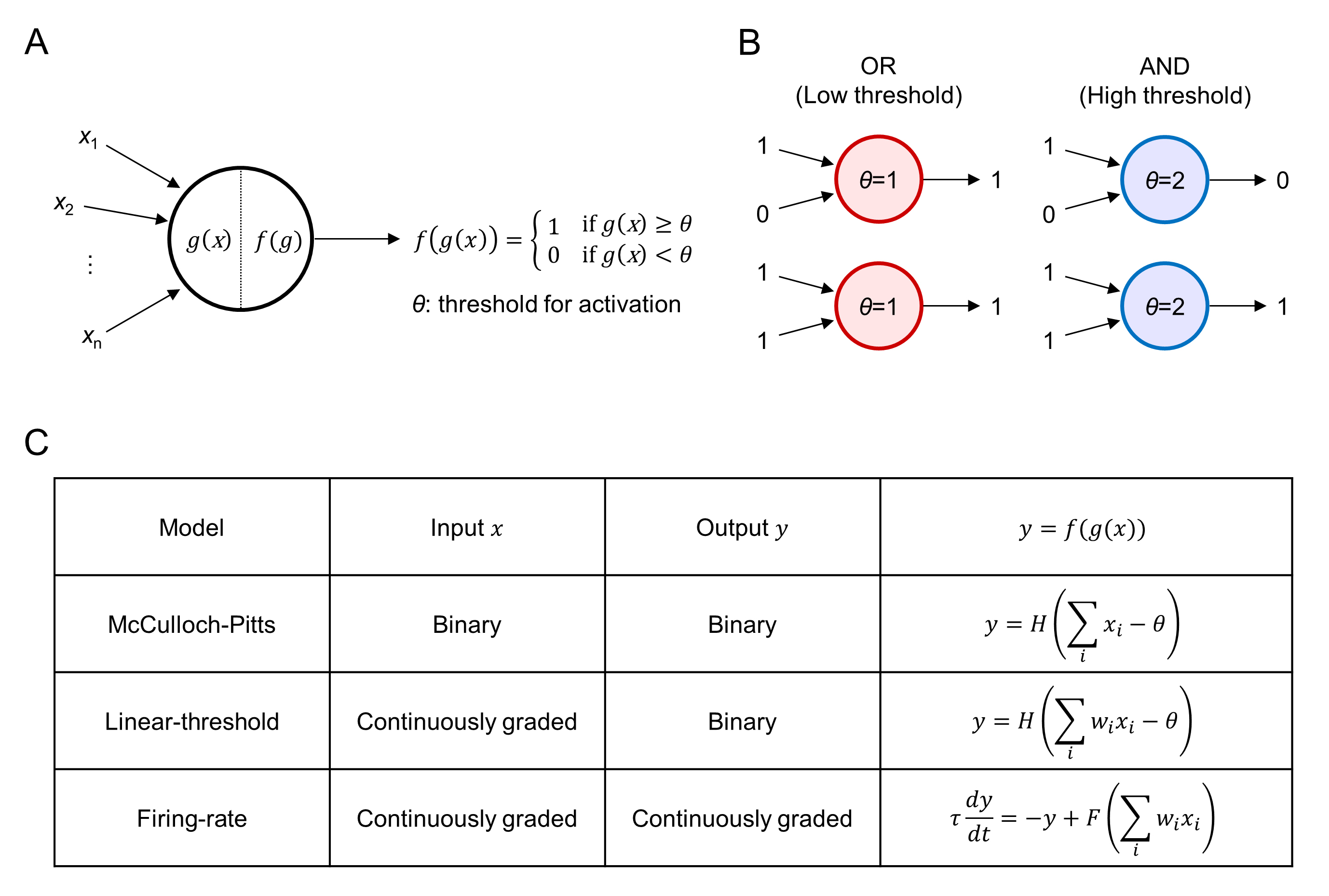 Fig. 1.
Boolean logic operations in simple neuron models. (A) Schematic
diagram of a simple neuron model with binary output upon synaptic inputs
x
The integrate-and-fire (IF) model is the most widely used simple spiking neuron model in artificial neural network algorithms [25, 32, 33, 34, 35]. It is a single-compartment model describing the dynamics of membrane potential, with the morphologies of dendrite branches and axons not explicitly included.
The one variable IF models describe the relationship between the time-dependent voltage V(t) and current I(t):
where
Two-variable IF models include the additional time-dependent adaptive variable
with constant a controlling the adaptation to voltage and
V
Table 1 lists the five models, i.e., LIF (leaky integrate-and-fire); QIF (quadratic integrate-and-fire) with and without an adaptive variable; EIF (exponential integrate-and-fire) with and without an adaptive variable.
| Models | Adaptation | Parameters | |
| LIF | No | t | |
| QIF | No | t | |
| QIF* (Izhikevich) | Yes | t | |
| EIF | No | t | |
| EIF* (AdEx) | Yes | t | |
| Abbreviations: LIF, leaky integrate-and-fire; QIF, quadratic integrate-and-fire;
EIF, exponential integrate-and-fire. Asterisk (*) denotes the model with an
adaptive variable. Parameters: V | |||
The information transfer capabilities are assessed in the information-theoretic
framework originally suggested by Denève and colleagues [37, 38, 39, 40, 41]. Fig. 2
illustrates the framework used in the present study. In brief, the binary hidden
state triggers a presynaptic neuron. Then the presynaptic neuron fires a spike
train via a Poisson process with the firing rate q
where
where the average, defined to be taken with respect to the probability measure p(x), may be estimated as the time average.
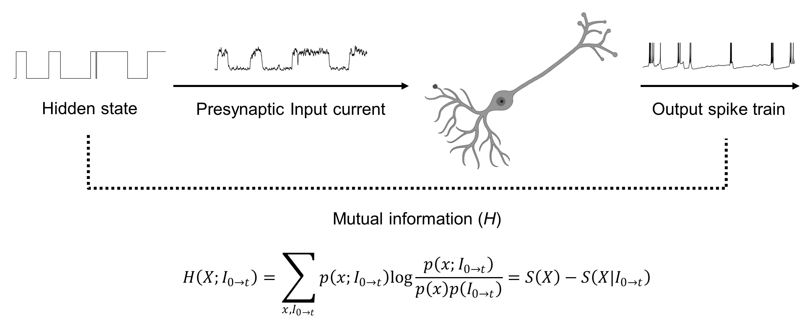 Fig. 2.
Illustration of mutual information calculation. The
binary hidden state triggers the presynaptic input current I. The mutual
information H(X; I
The conditional probability
where
The information-theoretic framework is used for comparing the neural dynamics
and coding properties of the five IF neuron models (Table 1). The train of hidden
state X is presented to each of the neuron models to induce the
presynaptic input current I and the resulting postsynaptic spike train
Fig. 3 displays the current-rate (I-f) curves (the left column) and the
time evolutions of the hidden state x and output spike trains (the right
column). The I-f curve, which expresses the relationship between the
applied current to a neuron and the firing rate (i.e., the frequency of output
spikes), is used as the basic measure for characterizing neural dynamics. The
firing rate f of the LIF model is the highest, followed by QIF and EIF.
The models possessing adaptive variables (QIF* and EIF*) exhibit reduced firing
rates compared with the corresponding models without adaptive variables. The
right column displays the time evolutions of the hidden states (the first row)
and resulting output spikes upon
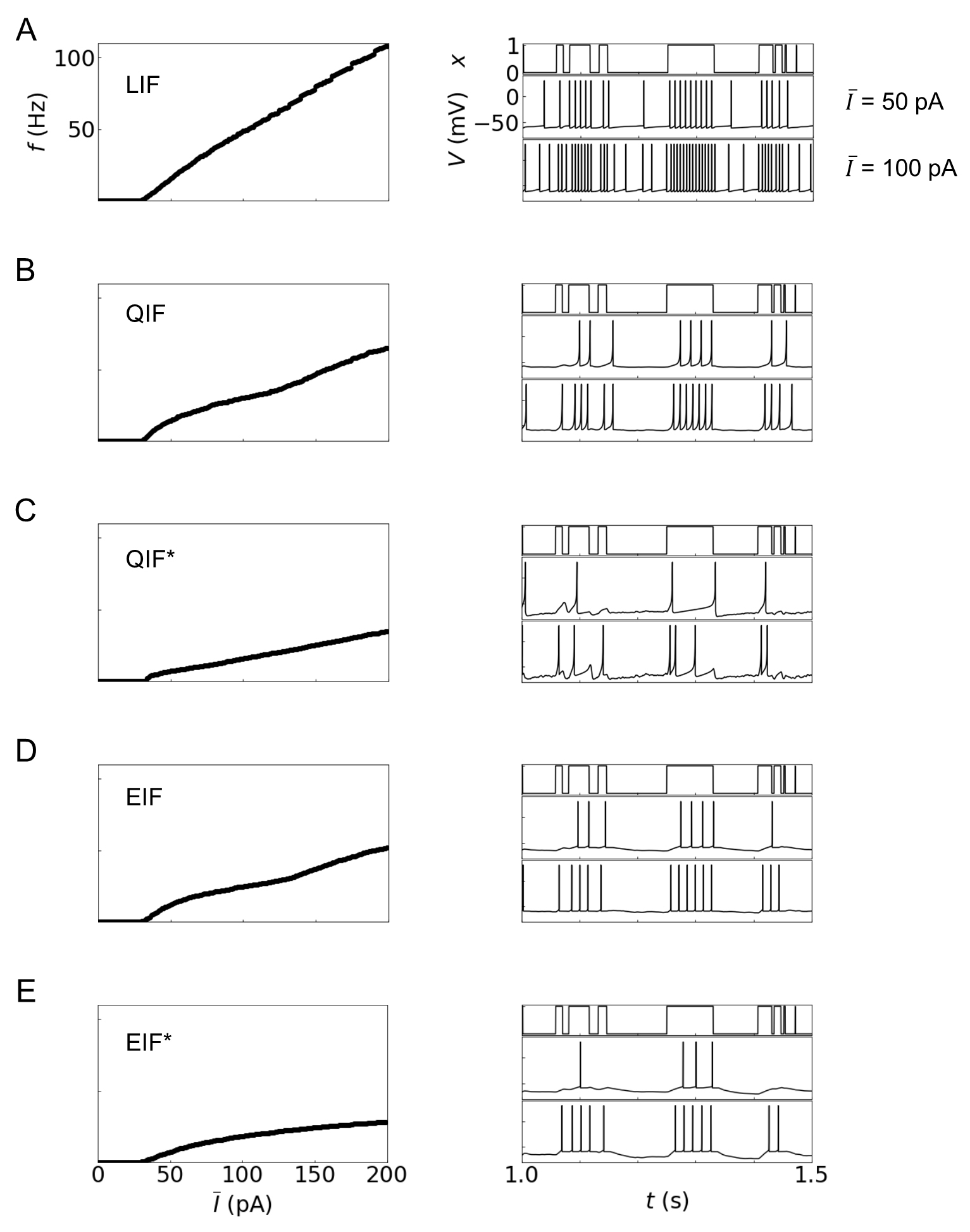 Fig. 3.
Dynamics of integrate-and-fire (IF) models: (A) LIF, (B) QIF,
(C) QIF* (QIF with an adaptive variable), (D) EIF, (E) EIF* (EIF with an adaptive
variable). The left column shows the I-f curves, where
The dynamics and information processing of IF models are mapped to Boolean
operations in Fig. 4. At a given threshold for firing rate f or that for
mutual information H, if f or H is greater than
or equal to the threshold, then the neuron is active (“1” or “true”); if it
is under the threshold, the neuron is considered as inactive (“0” or
“false”). Both OR and AND operations occur as a function of the fold change of
the difference between the threshold voltage V
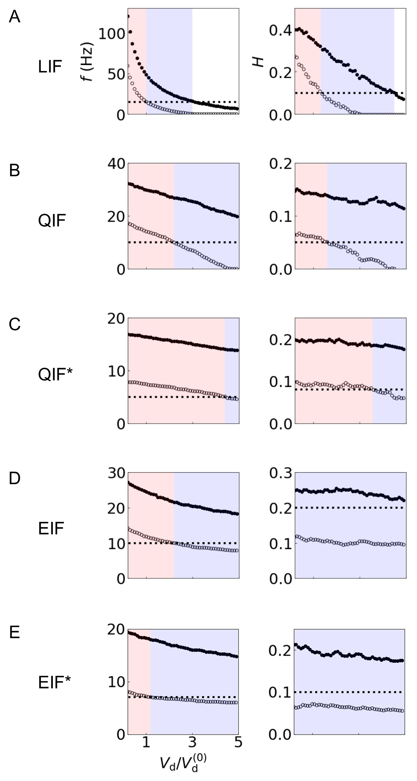 Fig. 4.
Mapping dynamics and information processing of IF
neurons to Boolean logic operation. (A) LIF, (B) QIF, (C) QIF* (QIF with an
adaptive variable), (D) EIF, (E) EIF* (EIF with an adaptive variable). The left
and right columns display the firing rate f and mutual information
H between the hidden state and output spike train, respectively. The
results for
Although these IF models are simplified versions of the biophysically realistic multi-compartment neuron models (which are explored in the following section), they appear to characterize the neural logic operations successfully. In particular, the neural dynamics and coding properties of exponential integrate-and-fire models (EIF and EIF*) are overall similar to the biophysical models, compared with other IF models [29]. The neural dynamics of IF models vary, depending on the mathematical form of the leak and spike-generating currents. In brief, the leak current term is necessary for responding to the changes of the hidden states in a timely manner; the IF models without the term usually fire in response to inactive hidden states (‘0’) because depolarization of the membrane potential during previous active hidden states (‘1’) is maintained during inactive states. The spike-generating currents [Eqn. 1 and Table 1] determine the speed of spiking: the IF models except EIF and EIF* exhibit much slower spike generation, compared with the biophysical model [29].
This section describes the characterization of information processing of the biophysically realistic multi-compartment neuron models, which describe how action potentials are initiated and propagated, based on Hodgkin-Huxley (HH) type conductance models for ion channels [43, 44]. Containing the axon and dendrites explicitly, the model has highly realistic structures via three-dimensional morphological reconstruction of biological neurons [45].
Two representative neuron models for neural computation are compared: the
pyramidal neuron in CA1 in the hippocampal circuit (ModelDB accession 7907) [46]
and PF in the cerebellum (ModelDB accession 7907) [46]. In the CA1 pyramidal
neuron model, all dendrites are divided into compartments with a maximum length
of 7 mm. Spines are incorporated where appropriate by scaling membrane
capacitance and conductance [47, 48]. Two Hodgkin–Huxley-type conductances
(g
The information-theoretic framework is similar to that used in Section 3 for IF
models, except that the stimulus sites are carefully chosen based on biological
knowledge and two inputs are provided simultaneously, with their competitive and
cooperative effects assessed [29, 50, 51]. Fig. 5 displays the schematic of the
framework. Each of the two hidden states X
In the rest of this section, we explore the information processing of homosynaptic plasticity (Section 4.1) and analyze Boolean logic operations triggered by one hidden state. Then we examine heterosynaptic transmission in the two hidden state scheme, which allows us to assess the synaptic cooperation and competition (Section 4.2).
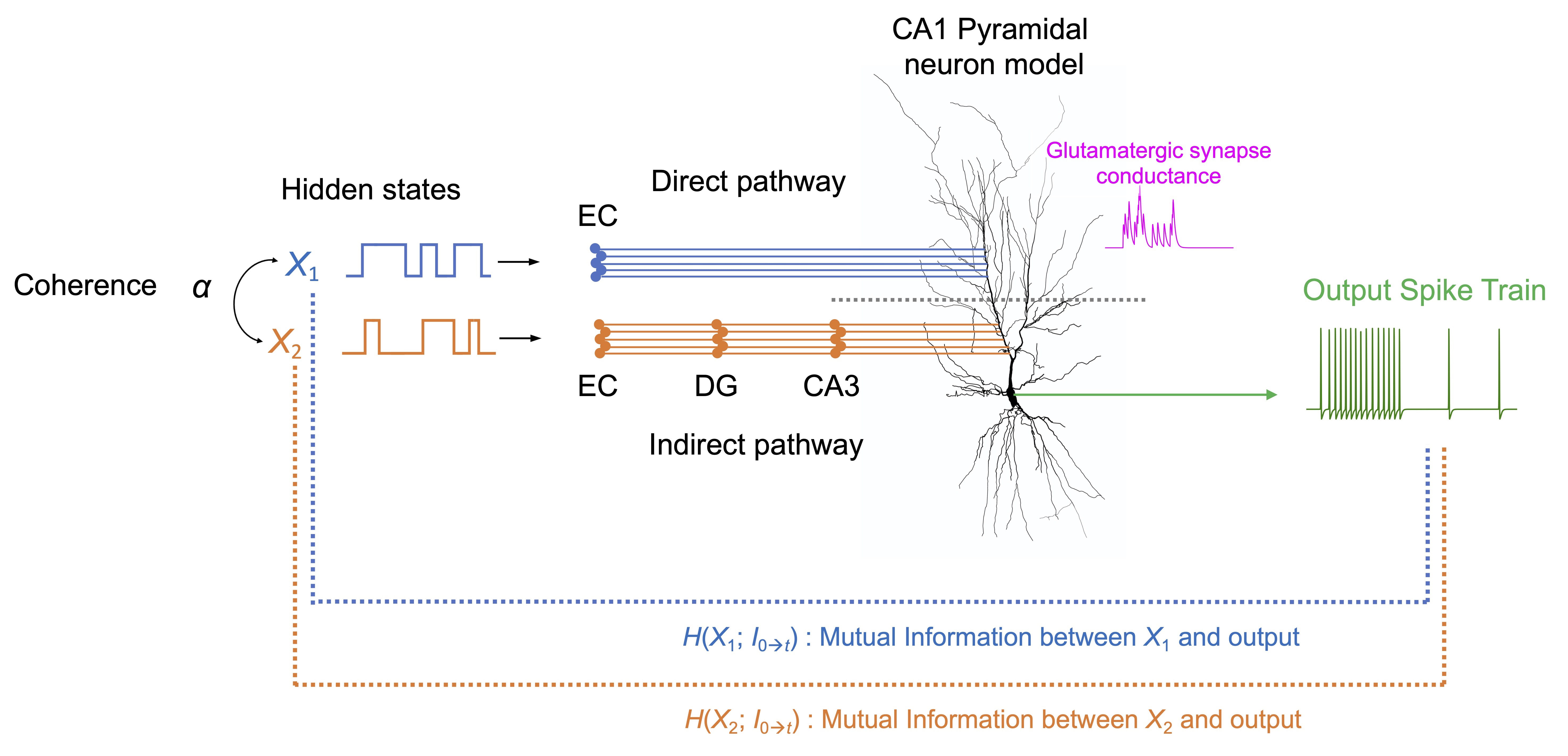 Fig. 5.
Schematic of the information-theoretic framework for multimodal
synaptic transmissions in the biophysical model of the CA1 pyramidal neuron.
Each of the two hidden states X
Homosynaptic transmission refers to the specific modification of a synapse by the activity of the corresponding presynaptic and postsynaptic neurons. The most widely used realization of this concept, first proposed by Hebb in 1949 [52], is the spike-timing-dependent plasticity (STDP) rule [53], which is often adopted in spike-based artificial neural networks. This rule states that a presynaptic stimulus immediately followed by a postsynaptic spike results in potentiation of the synapse while the opposite results in depression. Another well-known synaptic plasticity rule is the Bienenstock, Cooper, and Munro (BCM) rule [54, 55], according to which modification of the synapse depends on the instantaneous postsynaptic firing rate. In the original formulation of the rule, depression occurs when the postsynaptic firing rate is below a threshold while potentiation occurs when the rate is above the threshold. In particular, the threshold separating depression and potentiation is itself a slow variable that changes as a function of the postsynaptic activity.
Here, we implement a learning rule in which the STDP rule is combined with the
BCM rule [50, 56, 57, 58]. According to the STDP rule, weight changes occur for each
pair of presynaptic and postsynaptic spikes separated by time interval
where the subscripts p and d label potentiation and depression, respectively,
and
where
The BCM rule has a balancing effect that allows robust synaptic learning [55, 56]. The parameters for the learning rule are as follows:
Boolean logic mappings of the dynamics and information processing of the biophysical neurons are illustrated in Fig. 6. Note that the Boolean operations depend on the location of the synaptic input. For the CA1 pyramidal neuron, synapses are placed in the distal section or proximal section of the apical dendrite (a or b in Fig. 6A) in one setting or the other. These locations are selected based on neuroanatomical knowledge: The apical dendrite of the CA1 pyramidal has a long, extended structure to receive inputs from distinctly organized regions. Its distal region directly receives input via the perforant pathway from the entorhinal cortex while the proximal region indirectly receives via the granule cell and CA3 pyramidal neuron [59] (Fig. 5).
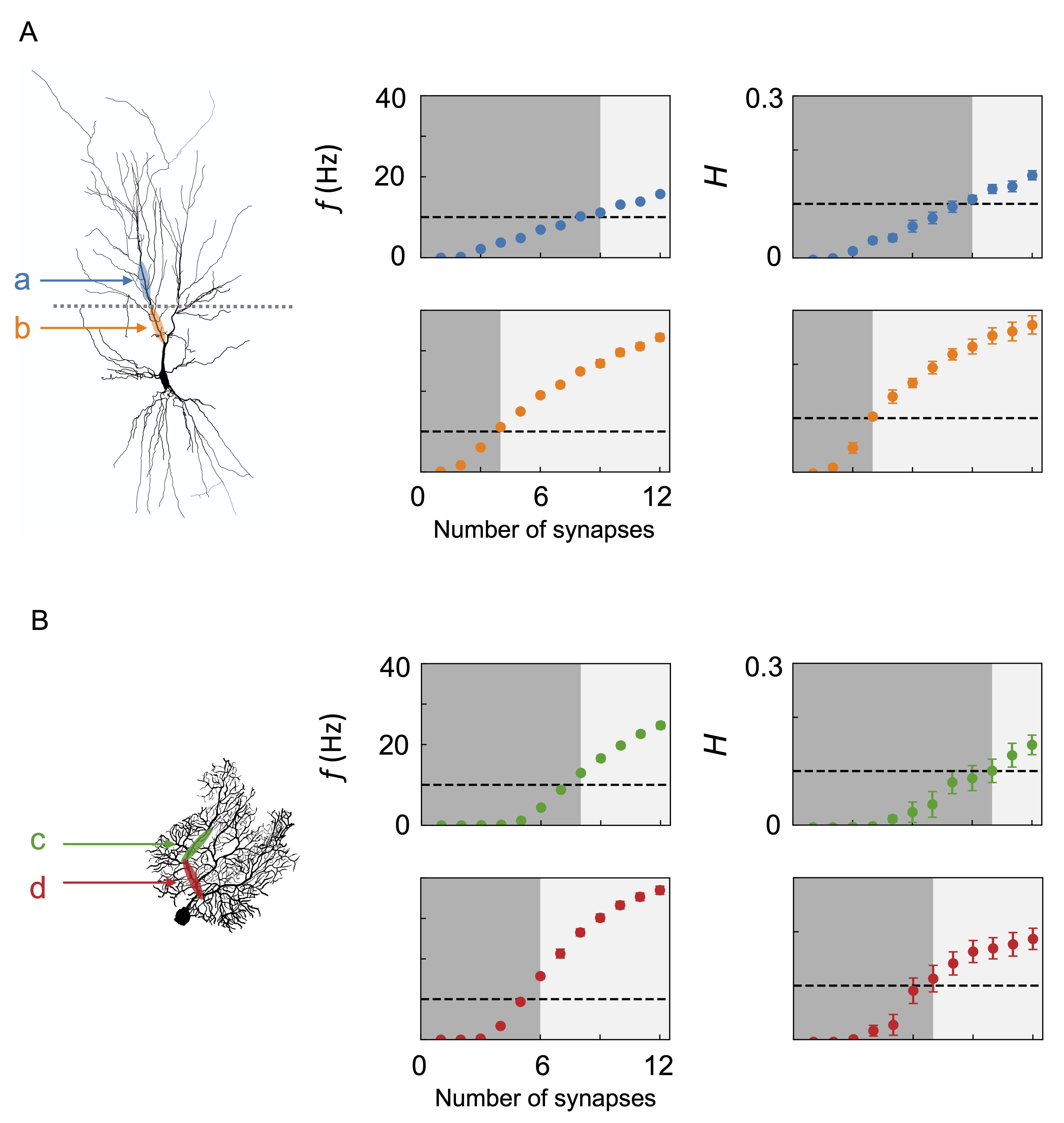 Fig. 6.
Boolean logic mapping dynamics and information processing of neurons: (A) CA1 pyramidal neuron and (B) Purkinje fiber. The morphologies of the neurons are illustrated on the left panels. The neurons are given synaptic inputs stimulated by a hidden state. For the CA1 pyramidal neuron, regions a and b denote locations of synaptic inputs placed relatively distally and proximally from the soma, respectively. For the Purkinje cell, locations of c and d correspond to relatively distal and proximal positions, respectively. The panels in the middle column show the postsynaptic firing frequency f as a function of the number of synapses in each condition. Those on the right show the mutual information H between the hidden state and the postsynaptic spike train. The outputs are mapped to Boolean operations using threshold values of 10 Hz and 0.1, indicated by the dashed line. When f or H is below and above the threshold, the output is zero (dark gray region) and unity (light gray region), respectively. Error bars represent the standard errors of five independent simulations with different random seeds for hidden state generation.
Presynaptic neurons fire at an average rate of 100 Hz, provided that the hidden state is on. When the stimulus is given to section a, nine synaptic inputs are required to cross the firing threshold of 10 Hz and the mutual information threshold of 0.1. In the case of the stimulus given to section b, the required number of synapses for the same threshold is just four. This manifests that the Boolean logic operations occurring with synaptic transmission depend on the location on the dendrite: in the distal region, the operation is closer to AND, with many concurrent inputs required to exceed the threshold, while in the proximal region, it is closer to OR, with only a few required.
The Purkinje cell has a highly branching, flattened structure built to receive inputs from up to 200,000 parallel fibers that pass orthogonally through the dendritic arbor [60]. In addition, each Purkinje cell receives input from one climbing fiber, which enwraps the dendrite and forms a vast number of synapses [61]. Unlike pyramidal neurons, there is no need for a vertical extension. Fig. 6B shows the logic operations performed by the Purkinje cell. Two inputs are given to two sections c and d along a main dendritic branch. The presynaptic neurons are assigned to a firing rate of 200 Hz when the hidden state is on. For the relatively distal section c, the firing rate threshold is crossed at eight synapses and the mutual information threshold at ten; for the relatively proximal section d the thresholds are exceeded at six and seven. Namely, there is a less drastic difference in the two sections compared with the CA1 case.
The CA1 pyramidal neuron and the Purkinje cell form well-established functional neural circuits that integrate multiple inputs from distinct sources. In particular, they can perform complex computation via homo and heterosynaptic mechanisms [50]. Heterosynaptic transmission refers to the modification of synaptic strength by unspecific presynaptic stimuli. The activity of a presynaptic neuron alters the strength of a synapse of the postsynaptic neuron not directly connected to the presynaptic neuron in action [62]. Unlike the homosynaptic case, there is no widely accepted computational model for heterosynaptic transmission.
The CA1 pyramidal neuron receives inputs mainly from two sources, one directly from the entorhinal cortex and one from the CA3 region [63]. The processing of these inputs is a critical step in the role of the hippocampus in memory, which is postulated to play a comparator role [64]. Synaptic plasticity in the CA1 neuron is well studied and exhibits rich heterosynaptic plasticity mechanisms [65, 66]. The Purkinje cell provides the sole output from the cerebellar cortex. It receives inputs from parallel fibers, axons of granule cells, and just one climbing fiber originating from the inferior olive, which nevertheless comprises about 1500 synapses. The Purkinje cell is believed to play a key role in motor learning, yet the synaptic mechanism remains elusive [67]. It was suggested in the early theories of learning in the cerebellum that heterosynaptic interactions between the parallel and climbing fibers play a key role [68, 69]. These neuronal systems have in common that heterosynaptic interactions between multiple inputs, which can be cooperative or competitive, play a crucial role in their computations [70, 71]. To understand the processing of these multiple inputs, we study them in our information-theoretic framework (Fig. 5).
Fig. 7 displays the Boolean logical operations of the neuron models at given two
multimodal inputs. For the CA1 neuron, X
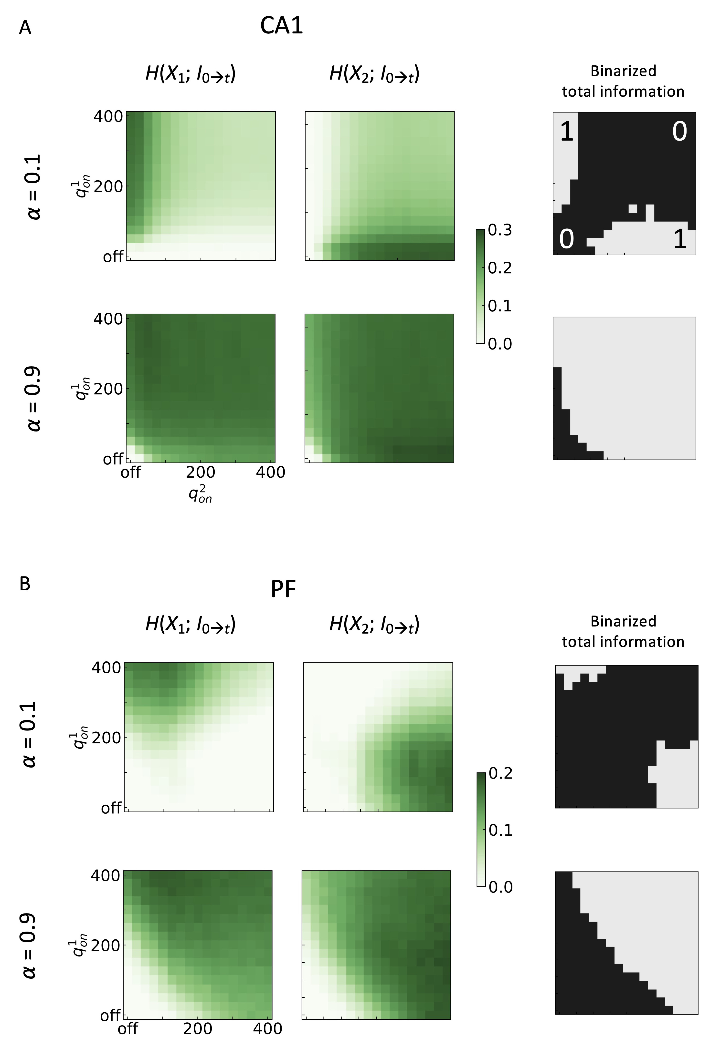 Fig. 7.
Information processing and Boolean logic operations of
multimodal synaptic transmissions in the (A) CA1 pyramidal neuron and (B)
Purkinje fiber (PF). The mutual information maps for
H(X
So far, we have discussed the characteristics and corresponding design principles for single neuron models and operators derived from small networks of neurons. In this section, we discuss the strategies to implement these models to a system of an even larger scale. Neuron models and logic gates play a crucial role in the dynamics of neural circuits. Algorithms inspired from neural circuits, such as artificial neural networks and variations, are also relevant despite its high-level representation of brain circuits, as the individual elements are technically an abstracted version of neuron models. As the scale and complexity increase, designing a performant and efficient circuit becomes more and more demanding. At its core, these systems can be interpreted as graphs with different types of nodes and edges. Then, the problem becomes to find the optimal topology best suited for a specific purpose. Often one might believe that finding the optimal topology is either unnecessary or inconsequential due to effectively no limitations available in the software representations of these systems. But this is not true for two reasons: First, the optimal topology is crucial for hardware design. Second, our brain does have limited resources, spaces, and connections with much more advanced motifs than those a typical learning problem might attempt to implement in software.
Optimizing the topological aspect of the model is a difficult problem and has garnered a lot of interest in various fields for quite some time. Here, we review two distinct fields that have made progress in applying computational algorithms to the physical systems to reconstruct or find the optimal topology. The two are the fields of systems biology and chip design: Systems biology, at its core, studies biochemical reaction networks inside a cell comprised of various enzymes and ligands. A computer chip, on the other hand, is a complex amalgamation of modules, subsystems, and logic systems. Once visualized, both can be represented using graphs and thus share similarities with neural networks and circuits. Both systems can be modeled and simulated as the basic dynamics of each type of building block are known. Due to the scale of the model and the diversity of elements and possible interactions between them, building a biochemical reaction network from scratch is difficult. Similarly, engineers have utilized various toolsets to aid the design process due to their complexity.
Current attempts at automated network topology design rely on one of several different techniques. Most prevalent is the inference techniques [72], with Bayesian inference being the most common of the bunch [73, 74]. Machine learning has become another popular choice, with examples such as optimization of biochemical reaction networks through machine learning [75], deep learning for regulatory networks [76], chip design using reinforcement learning [77], and sparse network identification using Bayesian learning [78]. There are also various information-theoretic approaches [79] using an ensemble of logic models [80], regression approaches [81], other heuristic, metaheuristic, and hybrid methods [82, 83, 84, 85], and many more.
Another approach, relatively less well-adopted, is the evolutionary algorithm (EA); it is a type of optimization algorithm that is heuristic and population-based. At its core, EA is characterized by concepts inspired by nature, with processes defined in correspondence to selection, reproduction, mutation, and recombination. An adaptation of EA may proceed as follows: (1) A population of individuals is initialized. (2) Fitness of individuals is evaluated. (3) Individuals are selected for reproduction, based on fitness. (4) Offsprings are generated with some probability of mutation and crossover. (5) The next generation is established with the number of the least fitted individuals reduced. (6) Repeat the process until the termination criteria are met. Many variations of the algorithm exist, most notably differential evolution and the particle swarm algorithm. While typically the algorithm is used for numerical optimization problems, it can also apply to inference and topology searching problems. We believe EA may provide several benefits over other approaches for automated designs of neural networks and neural circuits. The algorithm has garnered a lot of interest over the years on automated and optimal designs of artificial neural networks for learning tasks [86, 87, 88]. We suggest EA-based algorithms to be a good alternative for topological search and output optimization of neural circuit designs. Here, we give a short demonstration of finding an optimal set of functions to recreate a target output signal from the given input signals, examining the feasibility of circuit design automation via an EA-like algorithm (see Fig. 8). Technically, this version of the problem is not looking for different topologies per se but instead looking for the optimal set of transfer functions under a given topological constraint, which is imposed to make sure our example is analogous to neural circuits or neural networks. The workflow can easily incorporate topology modification with the adoption of an adjacency matrix-like representation of the topology. In this example, various predefined functions and logic operators are available for our algorithm to look for a model under some topological constraint that can mimic the output as much as possible. While we have used a set of elementary functions as the building blocks for demonstrative purposes, in more complex applications, they can always be replaced by more complicated classifiers, operators, layers, or even neuron models with detailed physiology specified. The contents of the building blocks can be of various scopes and levels of detail as long as an appropriate fitness function is chosen to reflect the changes.
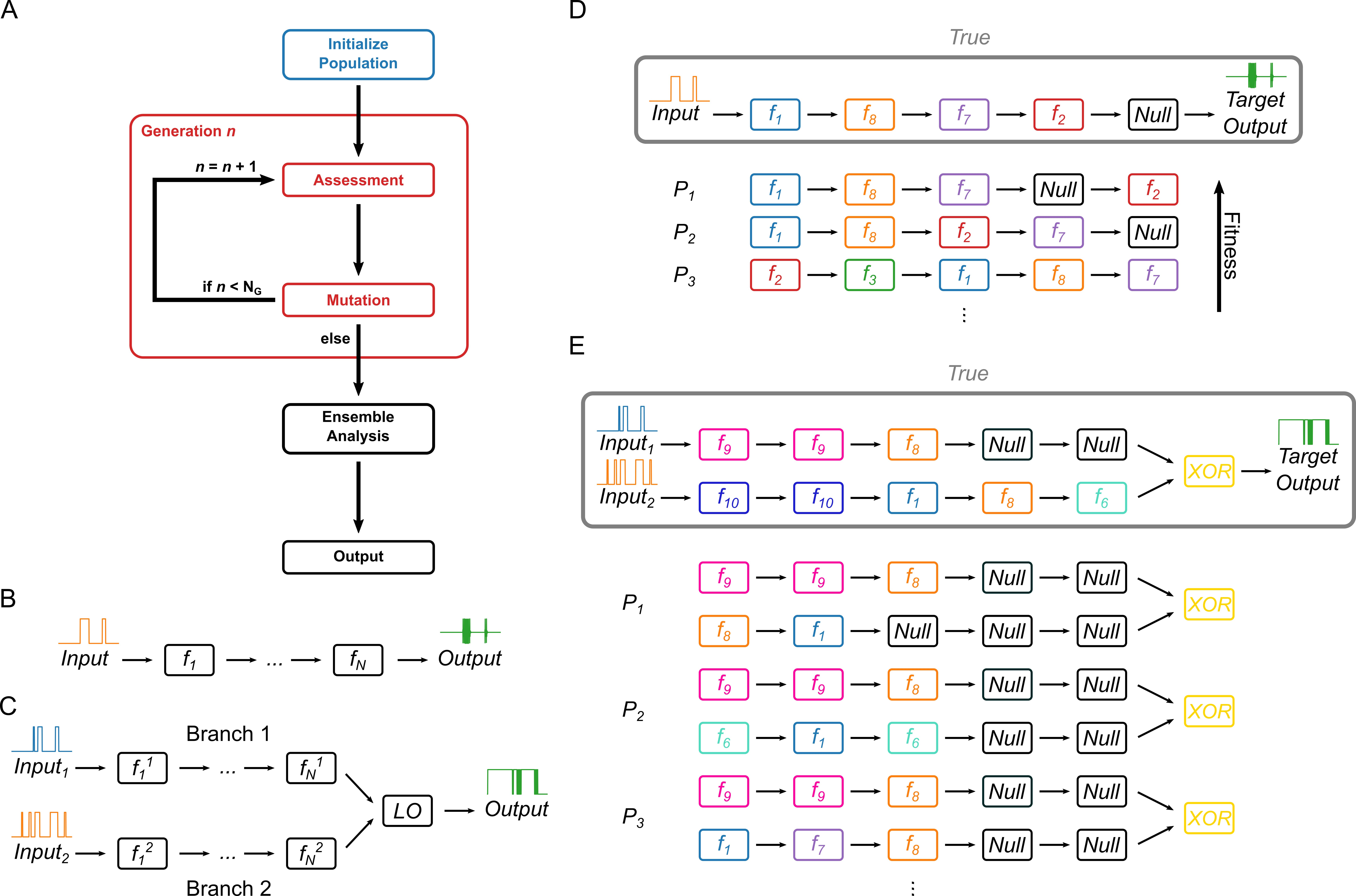 Fig. 8.
The demonstration of a framework for designing logic backbones.
(A) The overview of evolutionary algorithm. (B) Scenario 1, where a sequential
single-chain layer of functions akin to neural networks is used. (C) Scenario 2,
where two sequences of functions (branch 1 and branch 2) converge with a logical
operator simulating a multimodal neural circuit are used. (D) Result of scenario
1, where the output of the true sequence is given to the algorithm as the target.
The top three models with the highest fitness score are shown (P
For this study, we have created two different scenarios: one with a sequential
single-chain layer of functions conceptually akin to typical neural networks
(Fig. 8B) and the other with two sequences of functions converging with a logical
operator simulating a multimodal neural circuit (Fig. 8C). In each case, we
generate a synthetic model from which the target output is collected. For the
neural network example, we use the population size N
For scenario 1, we find that the algorithm recovered the original model nicely and collected similar models with comparable outputs (Fig. 8D). The multimodal neural circuit example is of particular interest since we believe neural circuit hardware design will benefit the most from the suggested approach. In the second scenario, multiple different models (N = 23) reproduce the given output. After analyzing the models, we notice that the differences are uniquely present in branch 2 while the algorithm recovers the correct logic operator and the sequence of functions for branch 1. We believe this is due to the binary nature of logical operators, where part of the information gets discarded. For a topology like Fig. 8C, where a logic operator integrates outputs from multiple sources, the content of the upstream elements might be tuned and simplified while keeping the desired dynamics, reducing the cost, therefore increasing the efficiency and potentially the scalability of the hardware implementation. Instead, the fitness function may be tweaked for parsimony, e.g., penalize a larger, more complex model, to achieve a similar goal.
The adjustment of edges (i.e., connections) between different nodes is crucial for the circuit design. Elements such as skip connections are known to have a profound impact on performance. A proper encoding strategy is necessary to achieve this goal. A directed graph representation is the most conceptually straightforward, with binary values indicating the connectivity between two nodes. For compartmental models, where the spatial aspect of synaptic plasticity may be studied, a continuous variable defining the position of synapses may be used instead. However, as many EA-based applications to neural network optimization for learning problems have demonstrated, a much more compact encoding is possible and recommended, as the initialization, mutation, and crossover can be performed much more efficiently. Support for variable-length encoding and artificial physical constraint are few other advantages. Another important factor in determining the performance of the algorithm is the evolving strategy. Crossover, in particular, is difficult to conceptualize for topology search. There have been algorithms such as NEAT [89] to address this problem. On top of mutation and crossover, artificially increasing the evolutionary pressure through the implementation of extinction/migration of individuals may be helpful for topological search, as the search space is discrete. On the same note, the application of generalized island models [90] may provide another interesting perspective to the problems with population diversity.
From the model engineering perspective, an EA-based algorithm like this is beneficial for two reasons. First, the algorithm, albeit optimized for the topology, is metaheuristic and therefore flexible enough to incorporate mechanistic models. Supporting mechanistic models indicates that detailed biophysics can be implemented in the bottom-up approach where both the models and the results are comprehensible for further analysis. This aspect of the algorithm is particularly valuable for the hardware design, where the implementation and debugging as much more straightforward. If an abstract byproduct of the model is used for the fitness score, an algorithm like this can provide a good balance between bottom-up and top-down strategies. Second, population-based optimization raises the possibility of collecting model ensembles. With a large population running for a long time, the algorithm can collect various models utilizing different strategies to achieve the same goal. Further, we can analyze an ensemble of different but equally good models to gain insight into the system. Additional constraints can be applied to obtain a reduced ensemble or a single model suitable for specific use cases. Another benefit of population-based algorithms is scalability, where massive parallelization is possible based on individual genealogy.
This study has investigated multiscale mechanisms of neural computation via computer simulations and information-theoretic analysis. We have first reviewed the operation mechanisms of three representative simple mathematical neuron models (i.e., MP, LT, and FR models) to introduce the basic concept of neural logic operations that might explain simple Boolean operations such as AND and OR gates. Next, IF models have been analyzed and the neural computations interpreted from the viewpoints of neural dynamics and neural coding approaches. These two complementary approaches allow a more comprehensive understanding of neural computation at the single-cell level. The analysis has extended to the biophysically realistic multi-compartment neuron models, which is adequate for evaluating versatile information processing through homo and heterosynaptic transmissions. We have then compared two representative multimodal neurons (i.e., the pyramidal neuron in CA1 in the hippocampal circuit and PF in the cerebellum), and finally, investigated the logic operations at the neural circuit level.
The simple neuron models (i.e., MP, LT, and FR models) are indeed beneficial for understanding the basic concepts of neural computations at the single-cell level. They successfully reproduce the basic single neuron behavior: neurons may have their own intrinsic thresholds for determining whether to fire or not, and this can be described with simple mathematical treatment. By introducing the Heaviside step function (for MP and LT models) or a differential equation (for FR model), these simple models can perform the basic Boolean logic operations such as AND and OR gates, in which the binary values 1 and 0 correspond to “true” and “false” (Fig. 1). Next, five IF models have been subjected to extensive simulations combined with the information-theoretic framework (Fig. 2). It has been manifested that both neural dynamics and neural coding approaches support the computational capability of neurons (Figs. 3 and 4). We have then investigated the role of synaptic transmission in neural computation through biologically realistic multi-compartment neuron models, and analyzed two representative computational entities, CA1 pyramidal neuron in the hippocampus and PF in the cerebellum in the information-theoretic framework. For single-input modalities, synapses proximal to the soma have turned out to act as OR gates whereas those distal to be closer to AND. This is particularly relevant in the CA1 pyramidal neuron, whose extended apical dendrites reach fibers from different sources. We have further assessed heterosynaptic competition and cooperation of the neurons at given multimodal inputs. Both AND/OR-like operations have been observed in the CA1 and PF for inputs with high coherence. On the other hand, when the coherence is low, both neurons exhibit the linearly non-separable XOR operation. This hints that complex computation can occur in single neurons, which may not be properly described by the simple neuron models.
For more complex circuits, algorithms that can design the optimal models for given requirements and constraints would be highly beneficial. For systems like neural circuits and neural networks, the optimization is performed in only a few orthogonal search spaces, e.g., parameter, dynamics, and topology. Network topology optimization is often overlooked, although it can have a profound impact on how the circuit performs. Note that in general different fields and subjects have different goals and limitations requiring different strategies. Systems biology, for example, is often bottlenecked by experimental limitations. Thus, constructing and validating against sparse data often presents a big challenge for systems biologists. We have demonstrated an example of an automated network design algorithm based on EA with two distinct design scenarios, and shown that despite the same algorithm and building blocks in both cases, the specificity of the ensemble differs vastly. While the linear chain example simply recovers the original model, the branched example demonstrates that multiple versions may satisfy our criteria in reconstructing the output from the given input. The population-based nature of EA can create an ensemble of equally good choices, from which the best is chosen based on the overall priority of the design principle.
The information-theoretic analysis used in this study is based on the method originally proposed by Denève and colleagues [37, 38, 39, 40, 41], which measures the mutual information between a hidden state triggering presynaptic inputs and the postsynaptic output spike train. This framework provides an ideal means to measure the information processing of a single neuron. Extending the method, we have included two hidden states to characterize the computation performed by a neuron receiving inputs from two information sources [29, 50, 51]. Since the seminal work of MacKay and McCulloch in 1952 [91] that first quantified the information contained in a spike train, numerous measures based on the classical information theory [21] have been devised to quantify information processing in single neurons and between neurons through synaptic transmission. Mutual information is a fundamental and versatile measure for the overlapping information between two quantities (e.g., presynaptic input and postsynaptic output) [17]. In our extended framework, two mutual information values are calculated for each input modality, allowing us to assess synaptic competition and cooperation.
The multiscale approach to neural computations presented in this study may provide a starting point for the design of biologically plausible neuron and synapse models in AI technologies. While most existing neuron models are designed as simple integrators of unimodal synaptic inputs based on the “dumb” neuron concept in the 1940s and 50s, recent experiments have hinted towards developing “smart” neuron models with potential applications in artificial neural network algorithms. In particular, linearly non-separable functions such as the XOR operation were traditionally thought to require multiple neuron layers and summing junctions [92]. A recent experimental study has shown that damping behaviors of the dendritic action potential in the neocortical layer 2/3 pyramidal neuron can perform XOR operations [15]. This result supports theoretical work that argued for complex computations at the level of single neurons [93, 94]. Moreover, there is growing evidence that such nonlinear functions at the single neuron level may provide an essential computational resource in neural networks [95, 96, 97, 98]. Large-scale deep learning algorithms have begun to explore complex operations at the single neuron level, such as the mirror neuron (for MirrorBot) [99], and multimodal neurons in the CLIP (Contrastive Language-Image Pre-training) algorithm [100].
In conclusion, this study describes simulations together with information-theoretic treatment of the multiscale logic operations in the brain. Both neural dynamics and information processing in biophysically realistic neuron models and phenomenological IF type models have been successfully mapped to the Boolean logic computation. Remarkably, neuronal information maps not only to basic AND/OR functions but also to the linearly non-separable XOR function, depending on the neuron type. Computational analysis on the multiscale nature of neural computation may be beneficial for understanding the computational principles of the brain and lay the foundation for developing brain-inspired advanced computational models.
Conceptualization, KH and MYC; modeling and simulations, JHW, KC, and SHK; analysis, SHK, KC, JHW, KH, and MYC; writing—original draft preparation, KC, SHK, JHW, and KH; writing—review and editing, MYC and KH; supervision, MYC and KH. All authors have read and agreed to the published version of the manuscript.
Not applicable.
Not applicable.
This research was funded by Korea Institute of Science and Technology (KIST) Institutional Program (Project No. 2E30951, 2Z06588, and 2K02430) and National R&D Program through the National Research Foundation of Korea (NRF) funded by Ministry of Science and ICT (2021M3F3A2A01037808). KC was supported by the KIAS Individual Grants (Grant No. CG077001). MYC acknowledges the support from the NRF through the Basic Science Research Program (Grant No. 2019R1F1A1046285).
The authors declare no conflict of interest.
AI, artificial intelligence; ATP, adenosine triphosphate; CA, cornu Ammonis; EA, evolutionary algorithm; EIF, exponential integrate, and, fire; FR, firing, rate; IF, integrate and fire; LIF, leaky integrate-and-fire; LT, linear threshold, MP, McCulloch and Pitts; PF, Purkinje fiber; PID, Partial information decomposition; QIF, quadratic integrate-and-fire.