
This study presents the classification of malaria-prone zones based on (a) meteorological factors, (b) demographics and (c) patient information. Observations are performed on extended features in dataset over the spiking and non-spiking classifiers including Quadratic Integrate and Fire neuron (QIFN) model as a benchmark. As per research studies, parasite transmission is highly dependent on the (i) stagnant water, (ii) population of area and the (iii) greenery of the locality. Considering these factors, three more attributes were added to the existing novel dataset and comparison on the results is presented. For four feature dataset, QIFN exhibited an accuracy of 97.08% in K10 protocol, and with extended dataset; QIFN yields an accuracy of 99.58% in K10 protocol. The benchmarking results showed reliability and stability. There is 12.47% improvement against multilayer perceptron (MLP) and 5.39% against integrate-and-fire neuron (IFN) model. The QIFN model performed the best over the conventional classifiers for deciphering the risk of acquiring malaria in different geographical regions worldwide.
Fifth-generation computing involves artificial intelligence (1). In the first generation, wires and switches were used, followed by transistors in the second generation, high-level languages (HLL) and integrated circuits (ICs) in the third generation, and code generators in the fourth generation. The fifth generation of computing introduced the concept of artificial intelligence (AI). In the present era of the computation, artificial neural networks (ANN) have gained significant attention due to their ability to quickly and efficiently compute. ANNs are inspired by the processing of information in biological nervous systems (2). ANNs are designed with highly complex interconnected information processing units (neurons) (3). The interconnection of neurons is dependent on the particular task of classification and/or pattern recognition. An ANN needs training for classification and pattern recognition. The learning process of an ANN is done by training to adjust the synaptic connections from one neuron to another, similar to biological neurons. The first mention of ANN occurred in 1943 in the work of W. McCulloch and W. Pitts (4). Since the McCulloch-Pitts (MCP) model, scientists and researchers have made many new sophisticated models, resulting in a new generation of ANN. In the MCP model, the neuron’s working was represented in terms of electrical Resistance-Capacitance (R-C) circuit response, as shown in Figure 1. Second-generation neural networks were fully connected networks that work through continuous input and output values. These neurons did not actually mimic biological neurons. They were rather inaccurate when compared with the brain’s neurons (5). To make neurons more efficient and accurate, biologically realistic models were developed to carry out computation. These third-generation neural networks, often termed Spiking Neural Networks (SNN), bridge the gap between machine learning and neurology (5). SNNs are fundamentally different in terms of operations and the working of basic units (neurons). SNNs work on distinct events over time in terms of spikes. Spiking events are mathematically represented in terms of a differential equation that represents the natural processes of neurons. The membrane potential is the most important feature of a neuron and is represented in the mathematical equation below. The occurrence of spiking events is dependent on the membrane potential; once this potential reaches a threshold value, it spikes and resets to a resetting potential. The integrate and fire neuron (IFN) model is the first implemented spiking model (6). The process of spike generation lasts for a short duration and produces a low amount of current, as given by:  , where
  is the capacitance,
  represents the fractional change in voltage with respect to time,
  and is the current (7).
 Figure 1
Resistance-capacitance equivalent model for IFN.
SSNs have been found to be more powerful than second-generation networks (8); it is natural to wonder why they are not widely used. The main challenge is the practical use of SNNs in training. Although unsupervised biological learning methods such as Hebbian learning and Spike-timing-dependent plasticity (STDP) have been utilized there are no known effective supervised training methods for SNNs that offer higher performance than second-generation networks. Due to the un-differentiability of spike trains, temporal information losses occur during the training of SNNs with the gradient descent method. Therefore, in order to properly use SNNs for real-world tasks, it is necessary to develop an efficient supervised learning model. This task is not easy, as it requires modeling how the brain actually learns.
On the one hand, SSNs are the natural successor of our current neural networks. On the other hand, they are quite far from being practical tools for most tasks; thus, the future of SSNs remains unclear. Some current real-world applications of SNNs include real-time imaging (9) and audio processing (10). Most papers on SNNs are either theoretical or show performance below that of a simple fully connected second-generation network (11). However, there are many teams working on developing SNN supervised learning rules, which indicate optimism for the future of SNNs.
Features play a vital role in classification and/or prediction tasks. Feature engineering is a technique for extracting domain knowledge from a dataset in terms of attributes. Predictive models are directly influenced by features. Better prediction results are directly proportional to the prepared and chosen features (12). There are several common methods for classifying data applied in almost every field of science.
Biomedical engineering is a popular area where classification and regression are applied. Several healthcare datasets are publicly available for research and development purposes. Some of the popular datasets used in research are Cancer data (13), Diabetes data (14), Heart disease data (15), Atherosclerosis data (16), Stroke data (17)(18), Lung cancer data (19), Brain cancer data (20), Breast cancer data (21), Liver cancer data (22)(23), Signal processing data (24), Skin cancer data (25), Primary tumor data (26), Blood cells data (27), etc.
Blood cells data is basically used for identifying infected blood cells and categorizing them as healthy or unhealthy. Malaria disease can also be predicted based on the information of blood cells. The features of blood cells have been analyzed by machine learning algorithms to classify cells as healthy or unhealthy. Malaria is one of the world’s most common life-threatening diseases.
This research involved the analysis of the effects of feature enrichment, the spirit of which comes from some of the work done by our group (28)(29).
Based on the attributes in the dataset, a neural network was trained, and then the proposed classifier was used to validate the prediction results. The focus was on changes in accuracy due to the increased number of features in the malaria dataset. A comparative study was performed to justify the results. This paper is organized as follows:
Section 3 presents work related to classification and feature enrichment found in the literature. Section 4 explains factors influencing malaria and mosquito species. Section 5 presents data set description. Section 6 showed light on classifiers: non-spiking and spiking. The experimental protocols are devised in section 7. The comparative study of the obtained results is discussed in section 8. Section 9 includes a detailed discussion on results. Finally, section 10 presents the conclusions followed by the acknowledgements and references.
Global warming is causing the number of insects and parasites that are responsible for spreading diseases in humans (30) to increase at alarming rates. The malaria parasite usually develops in semi-warm temperatures and stagnant water. Many stochastic and mechanistic models have been proposed in order to predict malaria. The most common approach to malaria prediction is using a metrological variable for fixed time duration to forecast abundance (31). Some researchers have proposed models based on rainfall and temperature variations (27)(32)(33)(34). Artificial neural networks are the most popular method for developing prediction models, especially in environmental studies (35) and bioinformatics (36). For malaria, symptomless carriers don’t require any treatment; however, they usually serve as reservoirs for the infecting parasites (37). Asymptomatic malaria incidences have higher potential to develop where improper treatments are done, as well as in places where environmental variables like temperature, rainfall, and humidity favor the development and growth of the parasite (38). India is one of the most malaria-endemic countries in southern Asia. Malaria is a life-threatening disease with a record rate of approximately one million cases per year and about 1200-1500 deaths reported in India. In India, malaria has spreading sequences, especially in the southeast. This study was conducted to identify the effects of climatic conditions, greenery, and population on malaria abundance in the south coastal region of India. Ponda is located in the South Goa district in the state of Goa with a latitude-longitude of 15.3991° N - 74.0124° E. Malaria incidences have been registered for the villages of Ponda, which has a tropical warm and wet climate and high humidity. The dense moist forest in this coastal region creates favorable conditions for the malaria parasite to develop and grow.
Apart from studies on malaria, some researchers have focused on the analysis of features and their impact on classifier performance. Authors in (39) presented a feature-enrichment method for textual data using sentence-level polarity classification and concluded that enriched representations give more accurate results and effective performance. Authors in (40) performed transductive classification on feature-enriched network data using test node features as training data for the classifier. They concluded that the mutual information-based feature-selection method shows better classification accuracy than collective content classification. Authors in (41) proposed a novel feature-enrichment method using the link analysis of short text-based classifications to select candidate words. Authors in (58) presented a feature-enrichment method for healthcare text classification using combinations of featured data and found improvements in the accuracy of classification using machine learning methods. Authors in (42) presented the significance of weighted feature enrichment and found it to be a better approach for hepatotoxic compounds. Authors in (43) presented a feature space enrichment method and found improvements in classification accuracy using a new approach rather than the original feature space. In this series, Authors in (44) presented a new feature enrichment method for face detection based on density parameters. Using density awareness in features yielded better accuracy and the authors advocated the use of density-aware feature enrichment in recent anchor design-based methods.
Based on these feature-enrichment processes, we hypothesized that the enrichment of features in the malaria dataset would lead to better prediction results over the original dataset. In machine learning applications, feature impact identifies which features (also referred to as columns or inputs) in the dataset give the best results. Features are considered effective if they are linear in behavior. The behavior of a feature affects outcomes like accuracy and sensitivity. Features that directly affect accuracy and sensitivity are considered predictors; features that do not affect them much are sometimes ignored in the feature selection method.
Malaria is commonly communicated through mosquito bites, but not all mosquitoes are carriers of malaria. Malaria is transmitted by female mosquitos of the plasmodium family. Mosquito bites are generally known for causing irritable itching. Mosquitos are generally divided by appearance into three classes (genera). The majority of mosquitos generally fall into three genera, but there are thirty-five hundred species and forty-one different families of mosquitos. Aedes, Culex, and Anopheles (the names were given by J. W. Meigen (45) in 1818) are three common genera of mosquitos discussed in this section. There are thousands of species of mosquitos worldwide; the three most significant are the aforementioned Culex, Aedes, and Anopheles, all of which transmit diseases. Out of the 460 recognized species, hundreds can transmit human malaria, but only thirty to forty common species transmit Plasmodium, which causes human malaria. Of the best-known genera, Anopheles Gambiae has a predominant role in the transmission of the most dangerous parasite species, Plasmodium falciparum (pF) (46). The breeding of mosquitos is mainly dependent on climatic conditions like temperature, rainfall, and humidity. There are many other factors that influence malaria transmission and growth. Apart from climatic conditions, stagnant water, greenery, and human populations play important roles in the development and spreading of the parasite. The three most dangerous species of mosquitos and other favorable factors are discussed below.
Several species of mosquitos are known to transmit vector-borne diseases in humans and animals. Dengue, malaria, yellow fever, chikungunya, Japanese encephalitis, West Nile virus, and tularemia are some vector-borne diseases carried by mosquitos. Hundreds of species of mosquitos can transmit malaria to humans (47). Below are discussed three of the most commonly found mosquito species in India that are known for spreading malaria disease.
Anopheles (45) mosquitos (shown in Figure 2A) are the most common breed found in fresh bodies of water that are surrounded by an abundance of wild plant life. Areas with still water, such as ponds, marshes, and swamps, are typical egg-bearing locations for female mosquitos. Anopheles is important to identify because they can spread the fatal disease called malaria. In particular, the Gambiae species transmits the deadliest form of malaria, known as Plasmodium Falciparum.
 Figure 2
Species of mosquito (A) Anopheles (B) Aedes and (C) Culex.
Aedes mosquitos (shown in Figure 2B) are anthropophagic, which means they only feed on human blood; this makes them especially dangerous (48). Aedes mosquitos are the most common species that spreads human diseases like yellow fever, dengue, malaria, periodic fever, and Lymphatic Filariasis. In certain cases, an illness caused by the bite of Aedes can lead to elephantiasis. This mosquito is mostly found in subtropical and tropical areas worldwide. Recently, this species has also been found in other warm areas, so it is expected to spread worldwide except to cold areas like Antarctica. Aedes females carry infections and transmit them to humans. Humans are more familiar with these mosquitos because the females prey on human blood. Aedes are also known as “floodwater” mosquitos because flooding is an important means for the egg-hatching process. Female Aedes lay eggs on the surface of stagnant water and the eggs become fully mature in six to seven days. The life cycle of Aedes mosquitos usually lasts about two weeks.
The Culex mosquito (shown in Figure 2C) is the most likely to spread malaria (49). Culex is not often associated with malaria in humans because these mosquitos prefer animal and bird blood over human blood. Due to this habit, they are not widely known for spreading diseases. Culex mosquitos are a diverse genus with more than 20 subgenera that includes thousands of species. Similar to the Anopheles mosquitos, Culex mosquitos lay eggs in stagnant water; however, they do not need to be surrounded by plant wildlife. Instead, they lay their eggs on outdoor objects that can carry stagnant water, such as barrels, cans, and garden pots. They carry deadly viruses such as West Nile and malaria.
The breeding, growing, and spreading of malaria depends on the climate (50). Climatic conditions like temperature and humidity play very important roles in the breeding and survival of mosquitos. India has various climates, including tropical, plain, and coastal regions. In some regions, the conditions are favorable for mosquitos. The coastal and sub-tropical regions are favorable for parasites. Areas with very low or high temperatures are not suitable for the breeding and survival of mosquitos.
Apart from these weather conditions, the distribution of malaria also depends on a location’s population and available greenery (51). Affected humans sometimes serve as sources to spread infections by means of mosquito bites. Once an uninfected mosquito bites an infected human, it carries the infection along with the blood and transmits it to another human through saliva. Stagnant water serves as a breeding ground for the parasite to develop and mature (52). People living in households surrounded by stagnant water are commonly infected by parasites. Stagnant water provides a more favorable condition for the lifecycle of mosquitos than does running water.
Knowing the three most common genera of mosquitos and the types of diseases they carry provides some insight into the relationship between the environment and mosquitos. When visiting these types of surroundings, it's important to take care regarding biting mosquitos and the infections they potentially carry.
This research involved testing the predictions of MD1 versus MD2. To do so required combinations of spiking and non-spiking neural classifiers. Cosine k-Nearest Neighbor (k-NN), Linear Support Vector Machine (L-SVM), Neural Time-series (NTS), Decision Tree (DT), Random Forest (RF), and Multilayer Perceptron (MLP) were the non-spiking classifiers. Integrate and Fire Neuron (IFN) and Quadratic Integrate and Fire Neuron (QIFN) were the spiking neural classifiers. A brief introduction to these classifiers is given below:
Non-spiking classifiers are well-known conventional linear and non-linear classifiers. A brief introduction to the non-spiking classifiers we used in this study is given below:
In classification and pattern recognition, there is an instance-based nonparametric learning method known as the k-Nearest Neighbor (k-NN) algorithm. In k-NN, the classification is based on a distance function (similarity measures). Classification is generally based on the predominance of neighbors, which are generally measured by a unique distance function (Euclidean, Manhattan, Minkowski, Cosine, or Chebyshev) (54). In general, the Euclidian function is used in k-NN, but once the distance function is cosine, it is termed Cosine k-NN. The distances functions for k-NN are listed below:
Euclidean:  (1)
(1)
Manhattan:  (2)
(2)
Minkowski:  (3)
(3)
Cosine:  (4)
(4)
Chebyshev:  (5)
(5)
where, “ ” is a dot product of vectors,
  are vectors or points and
  implies that
  is defined as (in contrast to “equal to”)
  .
.
The cosine distance method involves finding the angular distance between two vectors, while the Euclidean involves finding the distance. Figure 3 graphically shows the difference between the cosine and Euclidean distances, where  is the Euclidean distance and ‘
 ’ is the cosine distance.
 Figure 3
k-Nearest neighbour.
Support Vector Machines are supervised learning models associated with the analysis of data using learning algorithms (55). In a given set of training data, the members of each sample are marked in categories. The SVM training algorithm assigns each set to one category. The SVM represents the examples as points in a sample space so that separate categories are clearly separable through margins on the hyper-plane (as shown in Figure 4). Mathematically, it is represented as:
 Figure 4
Linear support vector machine.
 (6)
(6)
where,  is a vector, normal to hyper-plane and
  is the input vector. Some of the advanced applications of SVM can be seen in the recent publications (56)(57)(25).
A time series is a series of timely (equally spanned successive time intervals) and sequential recorded data points (59). Time-series analysis is a method for predicting future values in a dataset by analyzing past behavior. The analysis includes methods that extract useful characteristics and meaningful data. Past behavior includes previously recorded and analyzed values. There are two types of analysis methods: a) time-domain and b) frequency-domain. These methods may also be categorized as multivariate, univariate, nonlinear, and linear. When time-series data prediction is performed with the help of neural networks, it is termed a Neural Time Series (60). A model for predicting the future from relevant past values with delay elements and delay line is shown in Figure 5.
 Figure 5
Neural time series.
A decision tree is a widely used tree-based learning algorithm in supervised learning methods. These tree-type decision models have “test” and “outcomes” represented on an internal node and branches, respectively. A decision tree includes the modeling of decisions and possible outcomes, as well as utility, resource cost, and chance events. In the tree, class labels are represented as leaf nodes and branches are the outcomes of internal tests (nodes). Classification rules are obtained as the path from the root node to the leaf node (61). As seen in Figure 6, leaf nodes have a class label of true or false, intermediate nodes are decision nodes, and branches are the possible outcomes. Some of the good examples of DT-based methods can be seen in publications (62)(63).
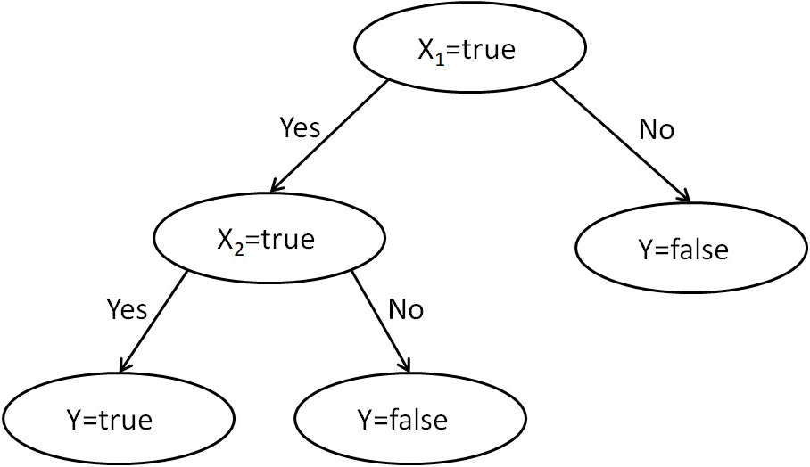 Figure 6
Decision tree.
Random Forest is an approach for the collective use of decision trees as a learning method for regression and classification. Trees are arranged and connected in a random subspace manner (64). A random forest combines the bagging idea and random feature selection approach (65). The preliminaries for a random forest include decision tree learning by averaging the multiple decisions of deep trees to reduce variance and bagging refers to bootstrap aggregation (66).
Several examples of random forest-based classification can be seen by our group (67)(68)(58).
Multilayer Perceptrons are feedforward neural networks with at least three layers: the input, hidden, and output layers (shown in Figure 7). Every neuron of the hidden and output layers has a nonlinear activation function to produce output. A Multilayer Perceptron involves backpropagation as a leaning method with the steepest descent error correction formulae (69). The most commonly used activation function for neurons is the sigmoid function (s-shaped), which is represented as:
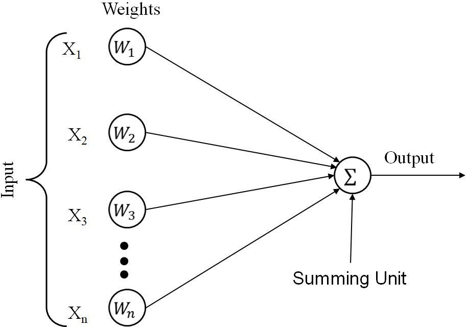 Figure 7
Multilayer perceptron.
 is the hyperbolic tangent function, and (7)
 is the exponential function known as a sigmoid function. (8)
The change in weights during error correction method is done by gradient descent method. The change in each weight is represented as:
 (9)
(9)
where,  represents the present layer,
  represent the previous layer,
  is learning rate,
  is output from previous neuron. The most recent example of MLP can be seen in the application given in (70).
Spiking classifiers are third-generation neuron models that are used as classifiers due to their efficiency, accuracy, and lower computational complexity. In this study, IFN and QIFN models were used to analyze the results rather than conventional non-spiking models. A brief introduction to spiking classifiers is given below:
The Integrate and Fire Neuron is the first-ever model that mimics biological neurons. The biological modeling of artificial neurons is known as spiking models, where nervous system functions are represented as electrical potentials (71). A neuron is represented as the time derivative of capacitance. When current is given as an input, membrane potential increases periodically and reaches a defined threshold; a spike is generated and voltage is reset immediately after the spike. This phenomenon creates a spiking pattern (shown in Figure 8) for a neuron that basically defines the scope and usability of that neuron. The capacitance model of IFN is represented as:
 Figure 8
Spike dynamics of integrate and fire neuron.
 (10)
(10)
where  is input current,
  is the membrane capacitance, and
  is the voltage at time
  .
.
QIFN is a special case of the generalized non-linear IFN model. The generalized IFN model was developed by adding the memory term in Eq. (11) to represent the ionic diffusion phenomenon, as occurs in the membranes of actual biological neurons. Diffusion takes place when the membrane cell is in a disequilibrium state. Generalized IFN is represented as below:
 (11)
(11)
where  is the membrane constant,
  is the membrane potential at time
  ,
,  is the leaky inductance of the membrane,
  represents the external input current, and
  and
and  represent the generalized functions of the membrane potential. We can obtain the QIFN by substituting a specific second-order function (
 ) for the membrane potential (
 ), which can be written as:
 (12)
(12)
where  is the leaky conductance of the membrane,
  is the resetting potential,
  is the threshold potential, and
  is the membrane resistance.
This section elaborates the methods used to bring this research in to the light. All the steps taken to carry the works, are explained in subsections including the datasets used in this study.
This study requires real time data for computations and observations, and to do so ethics approval were taken from Infectious Disease (ID) Hospital, Ponda, Goa, India. Dataset includes the information about the number of patients from a particular area (village). All patients who went through the test felt some symptoms of malaria due to mosquito bites, implying the presence of mosquitos in their locality. All manually kept records are digitalized in the hospital by staff and only spreadsheet records are taken to the Institute. The collected data contains the number of patients and their location (Village). We prepared the dataset using these records, along with the climatic conditions. The dataset contains five attributes: minimum temperature, maximum temperature, humidity rainfall, and the number of patients from each village. Historical weather details of Ponda, Goa were taken with permission under general public license from the URL:https://www.timeanddate.com/weather/@1259429/historic.
The Malaria dataset (MD1) contains the weather attributes and the number of patients. Climatic conditions play a very important role in the growing and spreading of mosquito-borne diseases. Temperature and rainfall are important factors for the breeding and incubation of mosquitos. Thus, these weather attributes were considered and mapped with cases from a particular village. The dataset was prepared for five consecutive years from 2013 to 2017 for all forty-three villages in Ponda. A sample dataset (MD1) is shown in Table 1.
| WN | Tmax (°C) | Tmin (°C) | Humidity (%) | Rainfall (mm) | # Patients |
|---|---|---|---|---|---|
| 1 | 30 | 17 | 55 | 3 | 52 |
| 2 | 30 | 17 | 56 | 4 | 62 |
| 3 | 31 | 17 | 55 | 14 | 45 |
| 4 | 32 | 18 | 62 | 12 | 45 |
| 5 | 33 | 19 | 60 | 5 | 32 |
The malaria dataset with five attributes was expanded to eight features by adding the population index, greenery index, and geographical index. The motive for adding these features was that these are also important factors for the spread of malaria (53). The population has a significant impact on the transmission of malaria, especially in localities where persons are migrating. Population migration can eliminate diseases or spread diseases to new areas. A sample expanded malaria dataset (MD2) is shown in Table 2.
| WN | Tmax (°C) | Tmin (°C) | Humidity (%) | Rainfall (mm) | PI | GI | Gr I | # Patients |
|---|---|---|---|---|---|---|---|---|
| 1 | 37 | 23 | 74 | 14 | 0.26 | 0.27 | 0.1 | 52 |
| 2 | 36 | 22 | 73 | 12 | 0.26 | 0.27 | 0.1 | 62 |
| 3 | 35 | 22 | 75 | 5 | 0.26 | 0.27 | 0.1 | 45 |
| 4 | 33 | 22 | 81 | 31 | 0.26 | 0.27 | 0.1 | 45 |
| 5 | 31 | 22 | 84 | 129 | 0.26 | 0.27 | 0.1 | 32 |
The collection of malaria data was given ethical approval from the Infectious Disease Hospital, Ponda, Goa, India. The patient records are maintained manually in the registers and these records were converted into computerized datasheets by the hospital before being transferred for this study. During the study, double-checking for errors was carried out after the data had been transferred from the hospital to the Institute. During computerization, the patient records were anonymized.
This section is divided into two subsections: the first section presents experiments using non-spiking classifiers and the second section presents experiments using spiking classifiers. Spiking and non-spiking classifiers were used to classify malaria-prone zones. Then, a comparative analysis of changes in the accuracies on different classifiers was performed. For this, the various experimental protocols were studied, as is briefly discussed below:
The aim of this experiment was to analyze the classification accuracy of the seven-feature dataset (MD2) and four-feature dataset (MD1) using the following criterion and to elaborate the effects and importance of an increased number of features for the incidence of malaria.
1. Linearly classifying support vector machines
2. Neural time series
3. Cosine k-Nearest neighbor method
4. Decision tree
5. Random forest
6. Multilayer perceptron
The aim of this experiment was to analyze the classification accuracy of the seven-feature dataset (MD2) and four-feature dataset(MD1) using the following models and to elaborate the effects and importance of an increased number of features for the incidence of malaria.
1. Integrate and fire neuron (IFN)
2. Quadratic integrate and fire neuron (QIFN)
Any of the research needs statistical validation for consistency and correctness in order to maintain reliability. The t-score, z-score and p-value tests are carried out. p-value test are meant to define the significance of a null hypothesis. p-values are the probability of unknown distribution of the random variable. t-test was carried out for four different data samples used. The obtained values are 3.69, 1.10 are for K2 and 22.08, -9.19 are for K10 protocols respectively for samples MD1 and MD2 datasets having 216 entries where the degree of freedom is 3 and 6 respectively. After this t-test, the p-value are obtained for one trailed hypothesis and found the significance in 0.5, 0.05, and 0.005. During the validations of hypothesis, the obtained p-values are 0.017, 0.175 are for K2 and <0.0001, 0.000042 are for K10 protocols for MD1 and MD2 datasets respectively, as given in Table 5. These values indicate that the significance of MD1 and MD2 datasets under K2 and K10 protocols under 0.5. MD1 dataset in K10 protocol found insignificant under 0.05 but MD2 dataset found most significant of all the three 0.5, 0.05 and 0.05. Least the p-value infers most the significance. Observed values are very close to zero which explains that the null hypothesis is strong enough to explain the observed values and adequately explain the observations on datasets.
This section presents the experimental results and is divided into three subsections. The first subsection presents the results for all enlisted non-spiking classifiers. The second subsection presents the results for spiking classifiers. The last subsection presents the comparative analysis. The computations were performed on a system with the following specifications: Intel® Xeon® CPU E5-2620 v4@ 2.10 GHz x-64-based processor, 16 GB RAM, NVIDIA TITAN XP 16GB GPU memory, and 64-bit Windows 10 (Professional edition). MATLAB R2015a was used as the computational platform. The symbols used in this paper are listed in Table 3.
| SN | Symbols | Description of symbol |
|---|---|---|
| 1 | Tmax | Maximum temperature |
| 2 | Tmin | Minimum temperature |
| 3 | η | Learning rate |
| 4 | τ | Membrane constant |
| 5 | gL | Leak conductance of the membrane |
| 6 | t | Time |
| 7 | Iext | External current |
| 8 | Vthres | Threshold potential |
| 9 | Vrest | Resting potential |
| 10 | V | Membrane potential |
| 11 | qi | Constant associated with aggregated function |
| 12 | I | Current |
| 13 | C | Capacitance |
| 14 | R | Membrane resistance |
| 15 | xi, yi | Coordinates (position) of selected point |
| 16 | k | Number of neighbours |
| 17 | • | Dot product |
| 18 | d | Euclidean distance |
| 19 | θ | Cosine distance |
| 20 | L(V), M(V) | Generalised functions |
| 21 | w̅ | Vector, normal to hyperplane |
| 22 | x̅ | Input vector |
| 23 | tanh | Hyperbolic tangent function |
| 24 | Yi | Output |
| 25 | °C | Temperature unit |
In this experiment, the MD1 and MD2 data were classified using non-spiking classifiers. To identify the effects of changing the number of features for the classifiers, 10-fold cross-validation (10 CV or K10) and 2-fold cross-validation (2 CV or K2) protocols were used as data shuffling methods for both datasets. Table 4 gives the results. Each classifier is discussed below:
| Dataset | LSVM | NTS | kNN | DT | RF | MLP | IFN | QIFN |
|---|---|---|---|---|---|---|---|---|
| K2 Protocol | ||||||||
| MD1 | 62.0 | 93.82 | 63.0 | 83.86 | 84.61 | 84.75 | 86.91 | 93.45 |
| MD2 | 88.4 | 94.51 | 88.29 | 92.76 | 89.39 | 82.96 | 87.16 | 94.45 |
| Mean | 75.2 | 94.16 | 75.64 | 88.31 | 87 | 83.85 | 87.03 | 93.95 |
| SD | 18.66 | 0.48 | 17.88 | 6.29 | 3.38 | 1.26 | 0.17 | 0.70 |
| K10 protocol | ||||||||
| MD1 | 71.68 | 96.73 | 72.73 | 88.24 | 87.17 | 87.11 | 89.81 | 97.08 |
| MD2 | 87.00 | 98.61 | 88.4 | 96.77 | 94.44 | 85.69 | 94.19 | 99.58 |
| Mean | 79.34 | 97.67 | 80.56 | 92.50 | 90.80 | 86.4 | 92 | 98.33 |
| SD | 10.83 | 1.33 | 11.08 | 6.03 | 5.14 | 1.00 | 3.09 | 1.76 |
Average accuracies for K2 protocol and K10 protocol were 62.0% and 71.68%, respectively, were obtained for the four-feature MD1 dataset and 88.4% and 87.00%, respectively, for the MD2 dataset. Standard deviation under both the protocols, for datasets MD1 and MD2 is observed to be 6.84 and 0.98 respectively. Figure 9 (A) shows a bar representation of the accuracies obtained for both protocols for the MD1 and MD2 datasets.
 Figure 9
Accuracies in K2 and K10 protocols using MD1 and MD2 (A) LSVM, (B) NTS, (C)k-NN, (D) Decision tree, (E) Random forest, and (F) MLP.
For NTS, we obtained average accuracies for K2 protocol and K10 protocol of 93.82% and 96.73%, respectively, for the four-feature MD1 dataset and 94.51% and 98.61%, respectively, for the MD2 dataset. Standard deviation under both the protocols, for datasets MD1 and MD2 is observed to be 2.05 and 2.89 respectively. Figure 9 (B) shows a bar representation of the accuracies obtained for both protocols for the MD1 and MD2 datasets.
For Cosine k-NN, we obtained average accuracies for K2 protocol and K10 protocol of 63.0% and 72.73%, respectively, for the four-feature MD1 dataset and 88.29% and 88.4%, respectively, for the MD2 dataset. Standard deviation under both the protocols, for datasets MD1 and MD2 is observed to be 6.86 and 0.07 respectively. Figure 9 (C) shows a bar representation of the accuracies obtained for both protocols for the MD1 and MD2 datasets.
The decision tree exhibited average accuracies for K2 protocol and K10 protocol of 83.86% and 88.24%, respectively, for the four-feature MD1 dataset and 92.76% and 96.77%, respectively, for the MD2 dataset. Standard deviation under both the protocols, for datasets MD1 and MD2 is observed to be 3.09 and 2.83 respectively. Figure 9 (D) shows a bar representation of the accuracies obtained for both protocols for the MD1 and MD2 datasets.
The Random Forest exhibited average accuracies for K2 protocol and K10 protocol of 84.61% and 87.17%, respectively, for the four-feature MD1 dataset and 89.39% and 94.44%, respectively, for the MD2 dataset. Standard deviation under both the protocols, for datasets MD1 and MD2 is observed to be 1.81 and 3.57 respectively. Figure 9 (E) shows a bar representation of the accuracies obtained for both protocols for the MD1 and MD2 datasets.
MLP exhibited average accuracies for K2 protocol and K10 protocol of 84.75% and 87.11%, respectively, for the four-feature MD1 dataset and 82.96% and 85.69%, respectively, for the MD2 dataset. Standard deviation under both the protocols, for datasets MD1 and MD2 is observed to be 1.66 and 1.93 respectively. Figure 9 (F) shows a bar representation of the accuracies obtained for both protocols for the MD1 and MD2 datasets.
In this experiment, the MD1 and MD2 datasets were classified using spiking classifiers. To identify the effects of changing the number of features for the classifiers, K10 protocol and K2 protocol were used as data shuffling methods for both datasets. The results for the classifiers are given in Table 4 and are discussed below:
IFN exhibited average accuracies for K2 protocol and K10 protocol of 86.91% and 89.81%, respectively, for the four-feature MD1 dataset and 87.16% and 94.19%, respectively, for the MD2 dataset. Standard deviation under both the protocols, for datasets MD1 and MD2 is observed to be 2.05 and 4.97 respectively. Figure 10 (A) shows a bar representation of the accuracies obtained for both protocols for the MD1 and MD2 datasets.
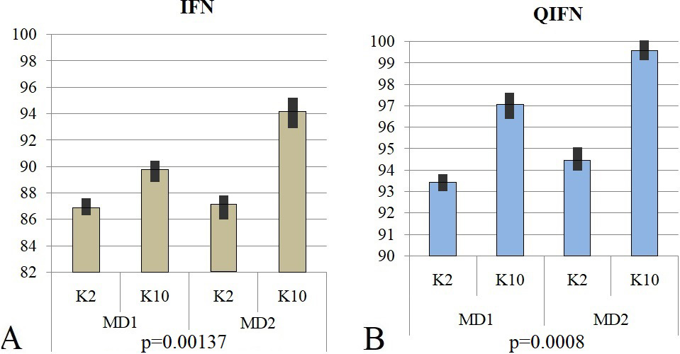 Figure 10
Actual vs. predicted malaria patients for the year 2016.
QIFN exhibited average accuracies for K2 protocol and K10 protocol of 93.45% and 97.08%, respectively, for the four-feature MD1 dataset and 94.45% and 99.58%, respectively, for the MD2 dataset. Standard deviation under both the protocols, for datasets MD1 and MD2 is observed to be 2.56 and 3.62 respectively. Figure 10 (B) shows a bar representation of the accuracies obtained for both protocols for the MD1 and MD2 datasets.
All the results obtained in the experiments point towards the performance capabilities of spiking neural networks. In linear classifier models, more improvements were noticed from changing MD1 to MD2, but spiking models exhibited efficient classification results on MD1. Some improvements in spiking models were also noticed from expanding the dataset. k-NN exhibited the highest improvements of 25.29% and 15.67% for the K2 and K10 protocols, respectively, when changing from MD1 to MD2. Adding significant features to the dataset increased the prediction accuracy of each classifier used in this study. Improvements of 15.32%, 1.88%, 8.53%, 7.27%, 4.38%, and 2.5% were found for LSVM, NTS, DT, RF, MLP, IFN, and QIFN, respectively.
The receiver operating characteristic (ROC) curve was used to validate the diagnostic capability of the SVM and k-NN classifiers. The plotted curve and the corresponding area under the curve (AUC) are shown in Figure 11. The AUC is 0.63 for both the SVM and k-NN for MD1 and 0.88 for both the SVM and k-NN for MD2. Thus, improvement in the AUC was seen from changing MD1 to MD2; this validates the hypothesis.
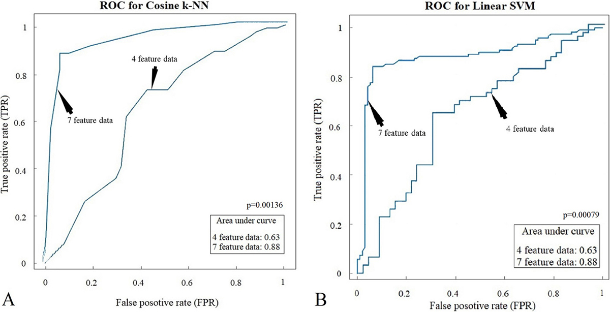 Figure 11
Receiver operating characteristics and area under the curve for (A) SVM and (B) k-NN.
Regression analysis is used to examine the association between two or more variables of significance. Regression for time-series analysis was performed; the training, testing, validation, and overall curves are shown in Figure 12. The figure shows that all data points are fitted as expected, with some acceptable errors.
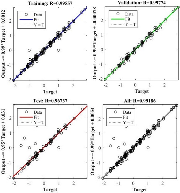 Figure 12
Regression plotting of neural time series.
For QIFN classifiers, the training, testing, and validation states using MD1 and MD2 are shown in Figure 13 and error graphs for MD1 and MD2 are given in Figure 14. The best validation performance for MD1 was captured at epoch35 and for MD2 at epoch5. The error graph shows that the system minimized errors in the third and fourth epoch and achieved stability for the MD1 and MD2 datasets.
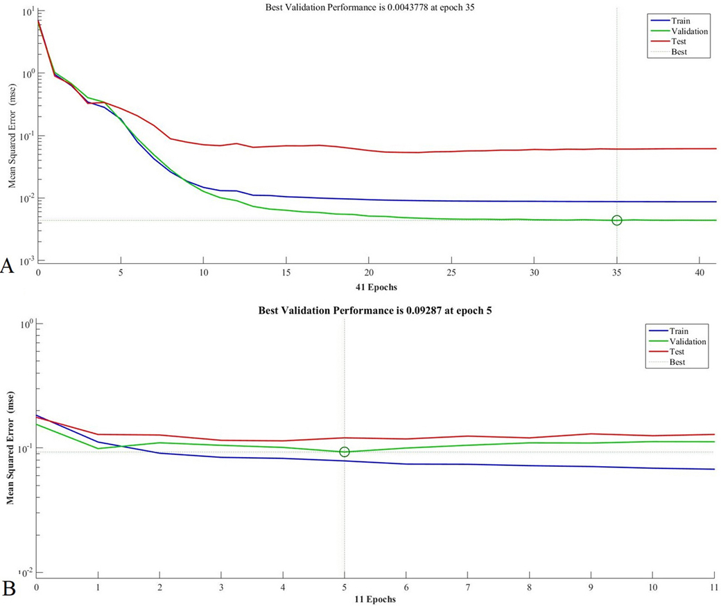 Figure 13
Training state of QIFN for (A) MD1 and (B) MD2.
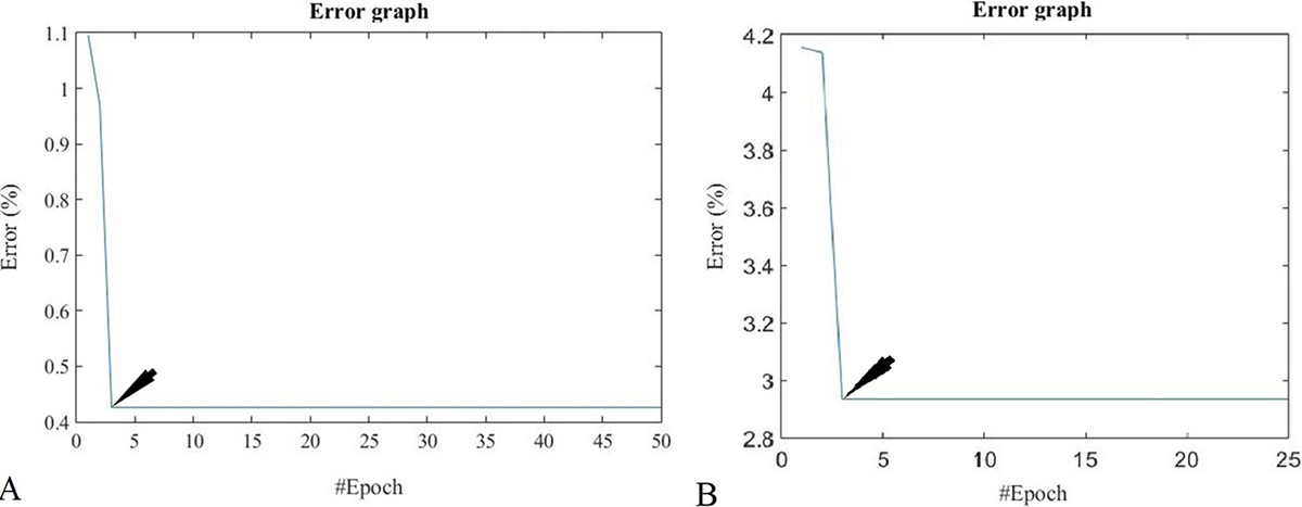 Figure 14
Error graph for QIFN for (A) MD1 and (B) MD2.
This study explores the effects of meteorological factors on the prediction of malarial incidence with the application of spiking neuron models. Two categories of models were used in this work: non-spiking (conventional) and spiking classifiers. Non-spiking classifiers comprise linear SVM, cosine k-NN, neural time series, MLP, decision tree, and random forest. The integrate and fire neuron model and quadratic integrate and fire neuron model were used as spiking models. Figure 16 provides a brief depiction of the overall work carried out in this study.
Initially, the study was performed on a collected malaria dataset (henceforth named as MD1) consisting of four attributes: minimum temperature, maximum temperature, humidity, and rainfall. QIFN exhibited superior performance compared to other classifiers, yielding accuracies of 93.45% and 97.08% for the K2 and K10 protocols, respectively using MD1. Further, the study was extended by increasing the number of attributes of MD1 from four to seven; this extended dataset was called MD2. These three additional attributes – population index (P. I.), greenery index (Gr. I.), and geographical index (G. I.) – were added because they are considered important factors in the spread of malaria (28). A survey study performed by the authors (28) suggested adding these features to the dataset to improve malaria incidence prediction. Similar studies were carried out for the MD2. For MD2, QIFN exhibited accuracies of 94.54% and 99.50% for the K2 and K10 protocols, respectively. Thus, QIFN improved accuracy by 1.09% and 2.42% for the K2 and K10 protocols, respectively, which further supports the justification of the work presented by authors in previous research (28).
The study was performed in a well-organized manner. Spiking and non-spiking classifiers were applied to MD1 and all observations were noted. Further, MD1 reconstructed and expanded to MD2 by adding three more features. The classifiers were applied to the new MD2 data set to investigate the effects of increasing the number of features on the classifiers’ accuracies. Impressive results were obtained; the performance of the classifiers increased and more accurate results were gained with this new dataset. Most improvements were seen for the K10, protocol implying that the system learns better with more instances in the training set. K-fold protocols mean the data is shuffled and divided into k-parts. K-10, or 10-Fold, implies that the dataset is divided into ten parts: one part was considered as a test set and the remaining nine formed a learning set; this procedure was repeated for all 10 parts. The average (or some other combination) classification of the ten testing sets represents the classification measure of the entire classifier. This was a complete iteration. These iterations were repeated many times; the data set was shuffled and a new complete iteration was performed.
For the different protocols and datasets, the Quadratic spiking model outperformed the other methods. As the number of attributes increased, better prediction results and higher accuracy were achieved. With a fewer number of features (dataset MD1), an accuracy of 94.54% was observed. After adding more features to the dataset (MD2), the accuracy increased to 99.58%. Thus, adding more features to the dataset makes it more efficient for prediction. This also proves that added attributes have a significant role in the prediction of disease. The performance of the QIFN was also evaluated using different combinations of malaria data. Monthly, half-yearly, annual, and five-year combined datasets were used for this performance evaluation. All the data preparation was carried out in an organized manner. First, the collected data was preprocessed and missing values treated at the hospital end. Training and testing datasets were created according to the K-fold technique: 10-fold cross-validation (10 CV or K10) and 2-fold cross-validation (2 CV or K2) were carried out. To validate the performance of the classifiers, receiver operating characteristics (ROC) were performed and plotted. It is clear that classifiers performance increased in terms of accuracy. The regression analysis shows that classes were classified correctly in order to predict new data of incidence. Under the spiking classifiers, the training, testing, and validation errors were noticed; errors were minimized and stabilized at the fourth iteration in both protocols.
Table 4 shows that QIFN showed minimum deviation (0.7 to 1.76) due to changes in the dataset for both the K2 and K10 protocols; k-NN has the highest deviation of about 11.08. Hence, QIFN was found to be more robust and trustworthy at malaria classification. Note that NTS the least deviation in the list of classifiers, but QIFN has better accuracy of classification. Thus, it was found that QIFN is the best candidate among the classifiers used in this study. During the experiments, all the classifiers improved from the increased number of features in the MD2 dataset, but MLP showed some disagreements in the K10 protocol and its accuracy decreased by 1.42%. Thus not every classifier improved from feature enrichment, though improvements were observed in most cases. Too many features can lead to the curse of dimensionality. The low number of features in our dataset called for an increase in features, which resulted in better classification for malaria-prone zones using spiking neural networks. Table 5 gives the information of t-test results and corresponding p-values obtained. Form the table, it is observed and form p-values analysis of 0.5, 0.05 and 0.005, most significance of MD2 is noticed where MD1 in found least significant of 0.05 and 0.005. This validates the hypothesis for increasing number of features in datasets. Increasing the number of features in dataset is making a good impact on accuracies and stability of model as statistical significance is found in extended dataset. All accuracies in K2 and K10 protocols including p-values are shown in Figure 15.
| Dataset \ Protocols | K2 | K10 |
|---|---|---|
| MD1 | 1.36E-2 | 7.96E-4 |
| MD2 | 1.49E-4 | 1.29E-4 |
 Figure 15
Accuracies including p-values for all classifiers in K2 and K10 protocols.
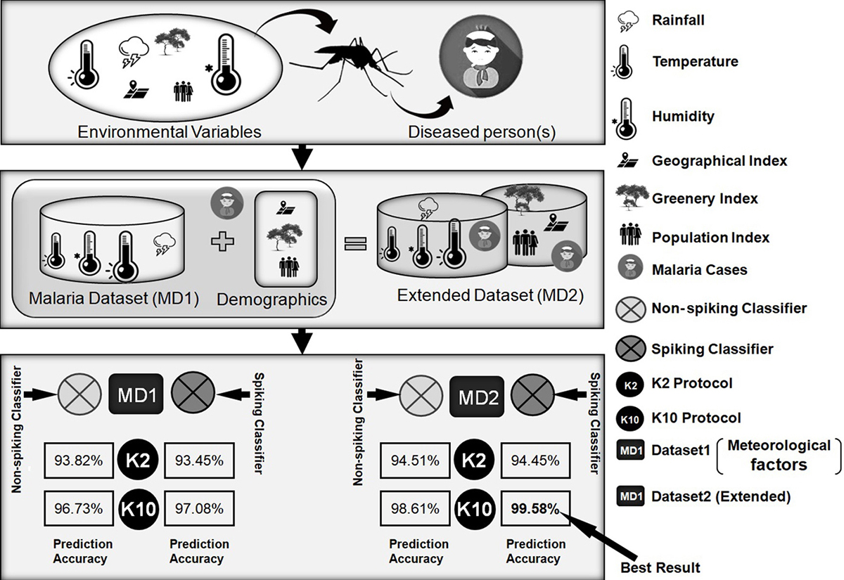 Figure 16
A brief depiction of the overall work carried out in this study
All the experiments and analysis showed that malaria-prone or non-prone zones can be predicted in terms of the average number of cases per year. Some of the villages were found to be prone to malaria from an increase in cases, but for the entire Ponda area, malaria cases decreased. Thus, it is concluded that Ponda is not prone to malaria. The dissimilarity index shows that the predicted results are quite efficient and accurate.
Features play a vital role in classification/regression. For any algorithm, the results and accuracy depend on the features of the data. Features are basically represented as columns in a dataset; among all the columns, one is treated as the response column of the target. Some datasets have too many columns (features), while others consist of a very low number of features. Having many features in a dataset makes it very rich, but also bulky, complex, and time-consuming to process using algorithms. In this case, the number of dimensions (features or columns) may need to be reduced; this is called Dimensionality Reduction. Datasets with few features need additional features to add more detailed information and obtain better results, as seen in this study.
Quadratic equations are widely used to model conceptual phenomenon. Quadratic equations are second-order equations and graphically represent parabolas, hyperbolas, ovals, and/or circle. In applied sciences, second-order equations are broadly used to represent the relationships of gravity and projectile motions. Second-order equations are also used in Coulombs Law, which relates the distance between charged particles, charge amounts, and electrostatic forces. Biophysical phenomena are nonlinear in nature and thus cannot be represented by linear equations; higher-order functions are therefore necessary. Second-order functions are also applicable to financial behavior modeling in the real world. Quadratic modeling meets the desired efficiency for accurately modeling biological phenomena.
Among all investigated classifiers, the quadratic model exhibited the best average results in all aspects. The quadratic model has a second order activation function, which means that it is best for representing biological neural activities. The scope of this experiment was limited to numerical data; because a limited amount of data was used, the results are concise and the scope is specific to the purpose. Better results were obtained after adding vegetation, geographical area, and population index as attributes. This type of modeling can also be applied to the prediction of other diseases like HIV, dengue, tuberculosis, etc.
This paper presents the significance of population, greenery, and geographical location in the prediction of malaria incidence. A dataset was expanded and the performance of the system was measured. The four-feature data was called MD1 and the expanded seven-feature dataset was called MD2. K-Fold techniques were used as the data shuffling method. K2 and K10 methods were applied to both MD1 and MD2datasets. Spiking and non-spiking classifiers were analyzed in order to compare the performance of the classifiers. This revealed the spiking models to be superior. Within the family of spiking neuron models, the Quadratic Integrate and Fire Neuron (QIFN) model exhibited outstanding performance. The results were better using the QIFN model on the MD2 data than on the original data, yielding cross-validation accuracies of 93.45% and 94.45% for K2 (50% training data) and 97.08% and 99.58% for K10 (90% training data) for MD1 and MD2, respectively. This shows an improvement of 2.5% for the K10 protocol for MD2. We conclude that the parameters included in MD2 have a significant role in incidence prediction and spiking models are more efficient than conventional classifiers.
We are thankful to the Department of Science and Technology, Science and Engineering Research Board, New Delhi, India for providing financial support through, Project No. ECR/2017/001074. We also thank Dr. Pradip Shinkre, Medical Superintendent, SDH, Ponda for providing data used in this study and Dr. Ashwani Kumar, Scientist-F & Officer-In-Charge, National Malaria Research Institute, Goa for his key suggestions to carry out the research. Special thanks to Global Biomedical Technologies, Inc., Roseville, CA, USA in support throughout the project, especially in experimental design, performance evaluation, and stability analysis.
QIFN
Quadratic integrate and fire neuron model
Malaria Dataset 1
Malaria Dataset 2
high level languages
integrated circuits
Artificial Neural Network (ANN)
Artificial Intelligence
McCulloch Pitts model
Resistance-Capacitance
Spike-timing-dependent plasticity
Spiking Neural Network
Integrate and fire neuron
Linear support vector machines
Neural time series
k-nearest neighbour
Decision tree
Random forest
Multilayer perceptron
Population Index
Geographical Index
Greenery Index