State-of-the-art review on deep learning in medical imaging

Send correspondence to: Jasjit S. Suri, Advanced Knowledge Engineering Center, Global Biomedical Technologies, Inc., Roseville, CA, USA and Stroke Monitoring and Diagnostic Division, AtheroPoint™, Roseville, California, Tel: 916-797-5942, Fax: 916-797-5942, E-mail: jasjit.suri@atheropoint.com

Front. Biosci. (Landmark Ed) 2019, 24(3), 380–406; https://doi.org/10.2741/4725

Published: 1 January 2019

(This article belongs to the Special Issue Genomic and cellular changes in the development and progression of cancer and other diseases)

Download PDF

Brower Figures

Cite

Abstract

Deep learning (DL) is affecting each and every sphere of public and private lives and becoming a tool for daily use. The power of DL lies in the fact that it tries to imitate the activities of neurons in the neocortex of human brain where the thought process takes place. Therefore, like the brain, it tries to learn and recognize patterns in the form of digital images. This power is built on the depth of many layers of computing neurons backed by high power processors and graphics processing units (GPUs) easily available today. In the current scenario, we have provided detailed survey of various types of DL systems available today, and specifically, we have concentrated our efforts on current applications of DL in medical imaging. We have also focused our efforts on explaining the readers the rapid transition of technology from machine learning to DL and have tried our best in reasoning this paradigm shift. Further, a detailed analysis of complexities involved in this shift and possible benefits accrued by the users and developers.

Keywords

Deep Learning

Medical Imaging

Classification

Segmentation

2. INTRODUCTION

The advent of deep learning (DL) (1) has spawned a new era in research and development in data science. DL has affected each and every sphere of life within a very short span of time. The most immediate effect can be felt in the field of image processing (2), robotics (3), computer games (4), natural language processing (5), self-driving cars (6) and many others. The immense popularity of DL is because of higher performance in comparison with other conventional algorithms. The performance of DL has steadily increased with advent of Big Data while it has remained static for conventional algorithms (7). The high performance ratio along with the easy availability of computer hardware such as graphics processing units (GPUs) and multi-core processor chips has made DL immensely popular among members of data science community (8). The foundation of DL lies in the formalization of the idea that all the functions of the brain are derived from the neural activity of the brain (McCulloch et al. (9)). The McCulloch-Pitts model of the neuron stands as a ground breaking exploration on the working of neural network that leads to the development of several other neural models of the brain i.e., perceptrons (10), feed-forward neural networks (11), feedback neural networks (12), etc. While the earlier networks were either single layer (input-and-output) or included single hidden layer (input-hidden-outputs), the DL paradigm takes advantage by using many layers or hidden neurons and layers to add depth to the network.

Learning in this context can be either supervised or unsupervised. In supervised learning, the algorithm is trained by human observer using training data and corresponding ground truth (GT), where at the end of training the algorithm learns to identify complex patterns. In unsupervised learning, algorithm learns to identify complex patterns and processes without intervention from human observer. There are many adaptations of DL for medical imaging as shown in Figure 1. Deep belief network (DBN) (13, 14) is a DL adaptation for unsupervised learning, where the top two layers act as associative memory. The important applications of DBN has been in the generation and recognition of images (15, 16), video sequences (17) and motion capture data (18). Autoencoder is a DL-based network used for unsupervised learning (19). Architecturally, the input and output layers of an autoencoder consists of same number of nodes with one or more hidden layers connecting them. It is specifically done to train the hidden nodes to encode the input data in a specific representation, so that the input could be regenerated from that representation. Thus, instead of conventional GT, input data is used to train the autoencoder. The convolutional neural network (CNN) (20) is a type of DL, which is specifically used in computer vision. It is inspired by the functioning of the animal visual cortex. Like the animal visual cortex, CNN’s exploit spatially-local correlation by enforcing a local connectivity pattern between neurons of the adjacent layers. There are many different types of CNN models available such as LeNet (21), AlexNet (22), GoogleNet (23), etc. It’s been seen that performance of DL-based system stagnates and then deteriorates rapidly with increase in depth. Deep Residual Networks (DRNs) (24) allow for an increase in depth without performance degradation. In this paper, we thoroughly discuss different DL methods and their applications in medical or radiological imaging.

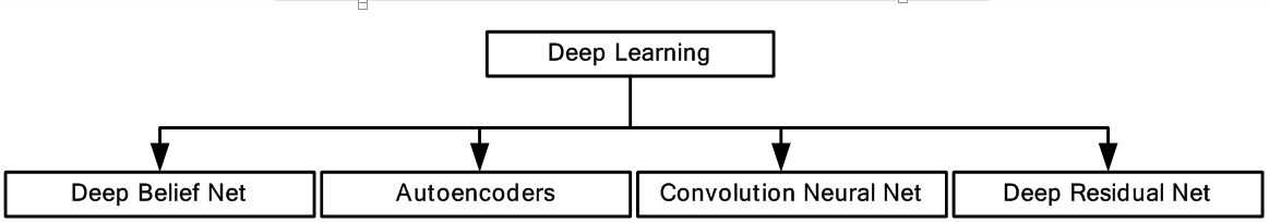Figure 1

Deep learning and its various adaptations.

In medical imaging, the scanned images of infected/abnormal regions are usually generated using computed tomography (CT) (25), magnetic resonance imaging (MRI) (26) and ultrasound (US) (27). Identification of infected tissues or any abnormality is generally done by trained physicians. The advancement of computer vision and machine learning (ML) has spawned a generation of technologies in computer aided diagnosis (CAD) of diseases. In this regard, in 2008, Suri developed an active deformable model (28) for cervical tumor delineation. In 2011, Suri and his team developed a feature-based recognition and edge-based segmentation for carotid intima-media thickness (cIMT) measurement (29). The same group also developed an ML-based technique for ovarian tissue characterization in 2014 (30). In the same year, an attempt was made to develop a CAD system for detection of Hashimoto thyroiditis on US images from a Polish population (31). In 2014, Suri and his team developed a system for semi-automated segmentation of carotid artery wall thickness in MRI using level set (32). The characterization process of ML involves the extraction of features from multiple feature extraction algorithms. These multiple features are combined in various ways for effective characterization by ML-based algorithms. The methods of feature extraction from digital images and their combination are usually not comprehensive, resulting in low accuracy. The emergence of DL in medical imaging has eliminated the need of feature extraction algorithms as the DL systems generate features internally, thus bypassing the low effective feature extraction stage. In segmentation, deformable models (33) are generally used for inferring the shape of infected/abnormal region in a medical image. However, the accuracy of deformable models is affected by the presence of noise or missing data in image and thus results in a poor border shape. DL applies pixel-to-pixel characterization for inferring the estimated shape of the infected/abnormal shape in an image. This allows the DL to provide an accurate delineation of shape. In ML, for 3D segmentation (34), 3D atlas feature vector is computed from each voxel (3D image unit) along with probability maps and then training/testing is done to delineate the inferred shape. Such estimation using feature vectors is task specific and may not be accurate for all type of 3D datasets. In DL, the feature extraction is done internally to estimate the location of the desired shape. Thus, DL provides a generalized mechanism for segmentation of 3D images which can also be extended to include 4D data such as video. During training, the DL weights are updated layer-by-layer unlike ML where weights are simultaneously updated. The layer-by-layer updating of weights helps in better training of DL systems. The primary focus of this study is to study different DL models for medical imaging and their applications. The whole concept of this paper to compare and contrast the DL models adapted in different field of medicine. Since the imaging modality differs from disciple to discipline, it is therefore important to understand how deep learning models are adapted. Even though the fundamental technology of deep learning might remain overlapping same, but the role of spatial information, temporal information, correspondence information, shape of the structure, purpose the application (diagnostic, therapeutic or monitoring) is kept in mind while building this deep learning review in mind. In this paper, we study various applications of DL in the field medical imaging related to cardio, neurology, mammography, microscopy, dermatology, gastroenterology and pulmonary.

The paper is organized as follows: section two provides the detailed analysis of four types of DL systems, section three gives details about the application of DL in medical imaging, section four describes the corresponding literature survey and conclusion.

3. DEEP LEARNING ARCHITECTURES

In here we briefly describe the various DL-based frameworks discussed in the last section.

3.1. Deep belief networks

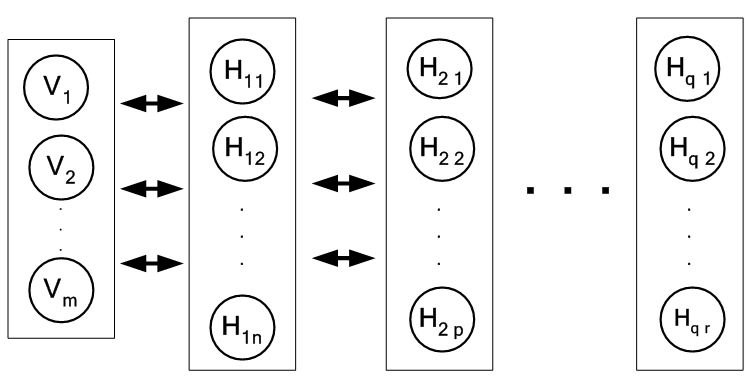Figure 3

A two-layer restricted Boltzmann machine.

Hinton’s (35) initial work on restricted Boltzmann machine (RBM) laid the foundation of DBN for classification, regression and feature learning. RBM is a two-layer network where the first layer is the input (also called visible layer) and the second layer is the hidden layer as shown in Figure 2. The joint probability distribution p under this model is defined by Gibb’s distribution which is given by:

$p (ν, h) = \frac{1}{Z} θ^{- E (ν, h)}$ (1)

where the energy function $E (ν, h)$ is given by:

$E (ν, h) = \sum_{i = 1}^{m} \sum_{j = 1}^{n} w_{i j} h_{i} ν_{j} - \sum_{j = 1}^{n} b_{j} ν_{j} - \sum_{i = 1}^{m} c_{i} h_{i}$ (2)

where, Z is normalization constant, $w_{i j}$ is denoted by the weight value between visible node $ν_{j}$ and hidden node $h_{i}$ and $b_{i}$ and $c_{i}$ are bias terms related to visible and hidden nodes. The nodes within a layer are not connected to each other, hence the term “restricted” which transcribes that, probabilistically the hidden node states $h_{1}, h_{2}, ... h_{m}$ are independent if input node states $ν_{1}, ν_{2}, ..., ν_{n}$ are given and vice versa. The independence between the variables allows states of all variables in one layer to be sampled jointly i.e., sampling of new state h for all hidden nodes is based on $p (h | ν)$ and sampling of state new state $ν$ for all visible nodes is based on $p (ν | h)$ which is also called block Gibbs sampling. These can be also represented as:

$p (h | ν) = \prod_{i = 1}^{m} p (h_{i} | ν)$ (3)

$p (v | h) = \prod_{j = 1}^{n} p (ν_{j} | h)$ (4)

Since learning in RBM is unsupervised, the probability distribution function $p (ν, θ)$ is considered the likelihood function of parameter $θ \in {W, b, c}$ for input vector $ν$ which can be also written as $p (ν, θ)$ . Each input sequence tries to revise $θ$ to increase the likelihood of $p (ν, θ)$ . The most common learning algorithm is the gradient descends method which employs $\ln p (ν, θ)$ as the log likelihood function. The parameters are revised along the gradient $\frac{\partial \ln p (ν, θ)}{\partial θ}$ to bring more learning efficiency. It is given as:

$θ (n + 1) = θ (n) + b * (- \frac{\partial 1 n p (ν, θ)}{\partial θ})$ (5)

By using the output of hidden layer in an RBM, as the input of visible layer to another RBM, a stack of RBMs can be created which effectively is the Deep Belief Network (DBN). A DBN is shown in Figure 3 consisting of one visible layer with m nodes and q hidden layers with n and p nodes for the first two hidden layers and r nodes for the last hidden layer. A couple of strategies for effective training of DBN were proposed. Those are: (i) layer-wise unsupervised learning where each RBM in a DBM is trained layer wise and (ii) fine tuning where a suitable classifier such as back propagation network is added at the end of DBN. Inference in DBN models is easy, however, assessing generalization performance of this model is difficult because probability of data under the model is known only up to a computationally intractable normalizing constant, known as the partition function. An estimate of partition function would help in controlling complexity and generalization of the model (36).

Figure 3

A multilayer DBN.

3.2. Autoencoder

Autoencoder neural network (37) like DBN is an unsupervised learning algorithm applying backpropagation for learning. In here, the number of target values are same as the inputs. A simple single hidden layer autoencoder network is shown in Figure 4. Interesting structures about the given data can be learned by putting constraints on the network such as limiting the number of hidden neurons. If the number of hidden neurons is less than the number of input neurons, then the network learns a compressed form of the input and possibly find relationship between the input features. Even if the number of hidden neurons is high, interesting relationships can be discovered by application of sparsity constraints (38). We describe here mathematically the autoencoder model as a generalized single hidden layer model:

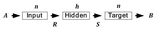Figure 4

A generic autoencoder model.

Let the number of input and output neurons be n . Let there be a single hidden layer consisting of h neurons. To generalize the working of $n - h - n$ autoencoder the following tuple $(n, h, m, P, Q, R, S, X, δ)$ where:

1. R and S are sets.

2. n and h are positive integers.

3. R is a class of functions from $p^{n}$ to $Q^{m}$ .

4. S is a class of functions from $Q^{h}$ to $P^{n}$ .

5. $A = {a_{1}, a_{2}, ..., a_{m}}$ is a set of m training vectors in $P^{n}$ . If external targets are present then $B = {b_{1}, b_{2}, ..., b_{m}}$ denote the corresponding set of target vectors in $P^{n}$

6. $δ$ is the dissimilarity function defined over $F^{n}$ is the dissimilarity function defined over .

Given any input, it’s the task of the autoencoder to convert a given input vector $a_{n} \in P^{n}$ to an output vector $R \cdot S (a_{n}) \in P^{n}$ . The task of optimization involves finding suitable candidate functions i.e., $r \notin R$ and $s \notin S$ to minimize the dissimilarity function $δ$ which is given by:

$\min G (R, S) = \min_{R, S} \sum_{i = 1}^{m} G (a_{i}) = \min_{R, S} \sum_{i = 1}^{m} δ (R \cdot S (a_{i}) a_{i})$ (5)

where, G is the overall distortion function. In here, the autoencoder tries to learn an approximation to the dissimilarity function where the output is similar to the input. In the case where both input and targets are provided, the minimization problem is given by:

$\min E (R, S) = \min_{R, S} \sum_{i = 1}^{m} E (a_{i}, b_{i}) = \min_{R, S} \sum_{i = 1}^{m} δ (R \cdot S (a_{i}) a_{i}) 1$ (6)

The derivation of features (36, 37) from the learned hidden neurons has been found useful in object recognition, vision and other non-visual tasks such as audio as well. One of disadvantage of using autoencoder is suffers from the problem of vanishing gradient. The vanishing gradient issue is thoroughly discussed in the next sub-section.

3.3. Convolution neural networks

Convolutional neural networks (CNNs) are simply neural networks that use specialized kind of linear operation called convolution in place of general matrix multiplication in at least one of their layers. CNNs are biologically inspired from Hubel’s work on a cat’s visual cortex (39). The visual cortex consists of a complex arrangement of cells sensitive to small sub-regions in the visual field. These cells act as filters over the input and exploit the strong spatially local correlation present in natural images. CNNs exploit this spatially-local correlation by enforcing a local connectivity pattern between neurons of adjacent layers. The basic building block of CNN consists of three operations which are: (i) convolution, (ii) rectifier linear unit or ReLu and (iii) pooling. Certain parameters such as convolution filter size, architecture of network etc., has to be defined before the training process. In the convolution stage, CNN applies convolution filters to extract features from the given input image. It preserves the spatial relationship between pixels by learning image features using small squares of input image data. CNN learns the values of filters or kernels during the training process. If a greater number of filters is used, then more image features get extracted from the given input image and our network becomes better at recognizingpatterns in unseen images. The convolution operation can be shown mathematically as:

$f (x, y) = I (x, y) Θ W (x, y) = \sum_{p = - \frac{m}{2}}^{\frac{m}{2}} \sum_{q = - \frac{m}{2}}^{\frac{m}{2}} I (x + p, y + q) \times W (x, y)$ (7)

where, image I is convolved with kernel W, yielding an output feature value f and $Θ$ represents the convolution operation. The convolution is basically the sum of all products between image I and kernel W , represented by Eq. 7, where the kernel is represented as a vector of size $m \times m$ and is shown for the point locations (x,y), while p and q are the dummy variables. After each convolution operation, ReLu operation is applied on the convolution output. In Artificial Neural Networks, gradient based methods learn a parameter's value by understanding how a small change in the parameter's value will affect the network's output. If a change in the parameter's value causes very small change in the network's output then learning is not effective which is also known as the vanishing gradient problem. In DL the problem becomes even more severe due to large number of layers. This is avoided by using activation functions which don't have this property of suppressing the input space into a small region. ReLu is a popular activation function which maps x to max(0,x). It is a non-linear operation where it replaces all negative pixel values in the feature map by zero. It is applied in CNNs to reduce the likelihood of the gradient to vanish. The pooling reduces the dimensionality of each feature map but retaining the most important information by using max pooling and average pooling. Pooling is done to simplify the output from CNN.

Multiple layers of convolution, ReLu and pooling are applied to extract high level features. Generally, a fully connected network (FCN) layer is appended at the end of the CNN for training and characterization purposes. CNNs have been widely used in computer vision tasks and are the most popular among all DL adaptations. CNN is used for both tissue characterization in medical images and segmentation purposes. However, the CNN requires large dataset for effective training. A variant of CNN called Fully Convolution Network (FCN) is specifically used for semantic segmentation discussed here.

3.3.1. A short note on fully convolution network

Fully convolutional network (FCN) indicates that the neural network is composed of convolutional layers without any fully-connected layers or MLP usually found at the end of the network. In FCNs, features are fused across layers to define a nonlinear local-to-global representation that is fine-tuned end-to-end. Each layer of data in an FCN is a three-dimensional array of size h x w x d, where h and w are spatial dimensions, and d is the feature or channel dimension. The first layer is the image, with pixel size h x w, and d is color channels. Locations in higher layers correspond to the locations in the image they are path-connected to, which are called receptive fields. FCNs are built on translation invariance. Their basic components (convolution, pooling, and activation functions) operate on local input regions, and depend only on relative spatial coordinates. The output of FCN represents high level or global features on which suitable classifiers are built by adding conventional classifiers such as perceptrons at their end which are basically CNNs. These features represent a coarse, downsampled model of the original image. These global features are upsampled and merged with intermediate low level or local features to give smooth segmentation maps of the original image

3.4. Deep residual network

With increasing depth of neural networks, they become more difficult to train. The accuracy saturates with a certain depth after which it degrades rapidly resulting in higher training error. Deep residual network (DRN) (24) simplifies the training of these networks, allowing networks to go to a greater depth. The notion here is that adding more layers should not increase the training error of its less deep counterpart. This notion is implemented mathematically as follows: Let’s say that $G (i)$ is a desired mapping from two stacked layers as shown Figure 5 (a). Then the residual mapping between the stacked layers is the difference between input i and desired mapping $G (i)$ i.e., $F (i) = G (i) - i$ as shown in Figure 5 (b). Then the original mapping is recast which is given by $G (i) = F (i) + i$ . The solution is shown Figure 5 (c). In this way, even if the training error does not decrease, it remains the same as its less deep counterpart. Also, the optimal mapping is closer to identity and easier to find small fluctuations. Therefore, training error does not increase with addition of more layers. Further, residual connections significantly reduced time for convergence. However, the deep residual network is used as a conceptual tool for enhancement of other networks rather than being a separate class of neural networks.

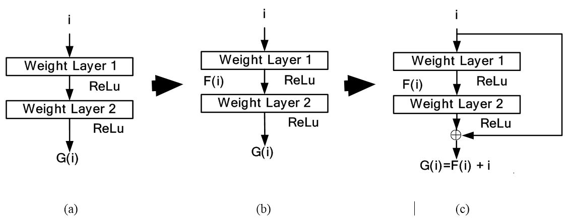Figure 5

Deep residual network conceptual model in subfigures: 5 (a), 5 (b) and 5(c).

4. DL-based medical imaging systems

The applications of DL in medical imaging have been rising rapidly. The independence of DL with regards to feature extraction has made it an attractive tool for imaging scientists, students and entrepreneurs alike. Many current tools which were dependent upon ML tools are increasingly shifting their focus to DL. There are a number of reasons for this shift. The first is the lack of identification of appropriate tissue characterization features for the various kinds of diseases. This can be attributed to the fact that ground truth data is not easy to collect due to the cost reasons. Typical ground truth data sets require manual delineations which can be expensive due to the time involved in manual tracings. Second, when histology and pathology ground truth is involved in 3D, this becomes very time consuming, very challenging and very expensive. This is typically seen in the component classification of plaques in the artery. Here the slices are cut perpendicular to the blood flow and thin enough to be seen in the microscope. Second challenge in the ML-based system is exhaustive search strategy needed for feature extraction with different kinds of frameworks. Each framework gives several set of features. Thus the combination of frameworks and feature size leads to 1000’s of features. Thus one needs exhaustive feature selection techniques which have detrimental effect on speed, learning, generalization effect, cross-validation protocol, etc. This adds large complexity in the ML-based systems.

Majority of DL applications for medical imaging fall primarily into two categories: (i) classification and (ii) segmentation. The generalized classification model is shown in Figure 6. Here, DL is used for characterization of medical images. As shown in the object process model the DL classifier is trained using GT of training data and finally tested with GT of test data. Depending upon the application, image segmentation can be sometimes more challenging compared to classification. This is because segmentation can involve a combination of classification followed by segmentation modeling. Classification can turn the images or volumes into different classes as an intermediate step, which can then be used for training the segmentation models. The trained models can then be applied to test data sets leading to the prediction of the segmentation of surfaces or boundaries. Thus in most segmentation problems, classification process are a precursor. For this reason, we are typically adaptive to intelligence based method for segmentation where one needs large spatial data sets. It is either done in one stage or two stages. In a one stage system, it is either done by a FCN or some pre-processing stage such as patching process. In patching, image patches are extracted which are manually annotated and then training/testing takes place. In the two stage system, segmentation generally involves rough estimate of the borders from the initial DL-based segmentation model trained using GT of training data. The second stage adapts a DL model or a conventional ML model to generate the refined output. The corresponding generalized two-stage segmentation model is given by Figure 7. This has been applied to many domains i.e. cardiovascular diseases, brain diseases, breast cancer, cellular biology etc. We present different successful applications of DL in different domains in the following subsections.

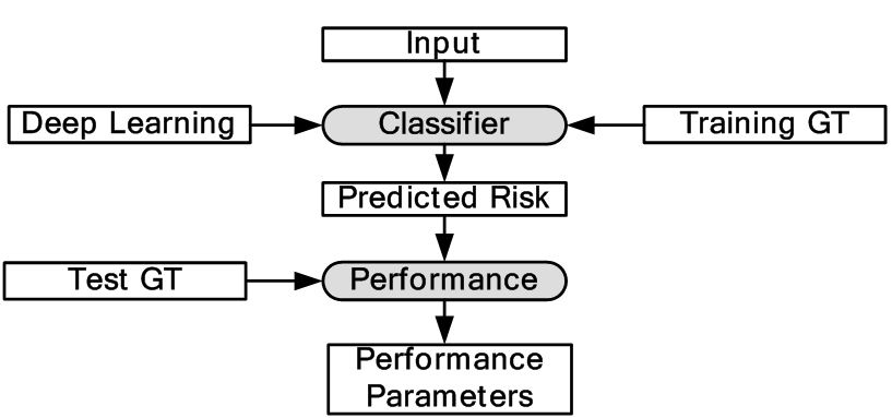Figure 6

Generalized classification model in DL framework.

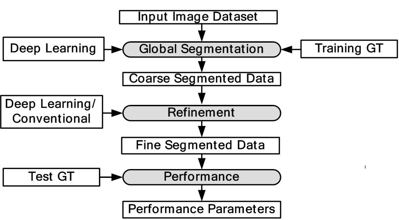Figure 7

Generalized two stage segmentation models in DL framework.

4.1. Cardiovascular application

DL has been widely used for left ventricle (LV) segmentation, vessel detection and plaque characterization. In here, we discuss five applications based on DL.

4.1.1. Tracking the left ventricle endocardium in US data

The two most important parameters to check the health of heart is ejection fraction measurement and assessment of the regional wall motion. These parameters can be obtained by the combination of segmentation and tracking of left ventricle (LV) endocardium from US scans of heart. Earlier attempts that were made to detect the size and contour using active shape and appearance model (32) but it had its own limitations. These models required a large annotated dataset for training, an initialization closer to local optimum, assumed a Gaussian distribution of shape and appearance from training samples which are not always accurate. Further, they did not consider priors which are important to capture all variations of wall motions. To resolve these issues, a new pattern recognition (40) approach for the problem of left ventricle tracking in US images is performed using DBN framework. The expected segmentation of the current time step t considers all previous segmentation contours c and current images produced. The author has defined current image I is a set of prior states where each state is defined by heart functions of systole and diastole i.e., $k = {systole,diastole}$ and the contour c which defines the shape. In this respect, given the cardiac phase and contour, the shape model can be described probabilistically as:

$p (I_{t} | k_{t}, c_{t}) \approx p (k_{t}, c_{t} | I_{t}) p (I_{t})$ (8)

where, $p (I_{t})$ is constant and $p (k_{t}, c_{t} | I_{t})$ can be described as integration of affine detection $p (k_{t} | θ, I_{t})$ , non-rigid segmentation $p (c_{t} | θ, k_{t}, I_{t})$ and prior distribution of affine parameters $p (θ | I_{t})$ :

$p (k_{t}, c_{t} | I_{t}) = \int p (k_{t} | θ, I_{t}) p (c_{t} | θ, k_{t}, I_{t}) p (θ | I_{t}) d θ$ (9)

where, $θ$ denotes parameters of affine transformation, $k_{t}$ represents the cardiac phase and $c_{t}$ is the LV contour. Thus, to estimate contour segmentation $c_{t}$ and cardiac phase $k_{t}$ , the affine transformation $θ$ has to be marginalized using the prior information estimated from the training dataset. A team of four cardiologists and one technician traced the left ventricle (LV) borders of 496 images dataset. The results were computed on 132 images. The traced images formed the GT of the experiment.

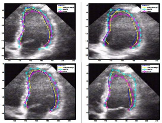
The model as described in Eq. 8 and Eq. 9, is implemented using two separate DBN-based architectures. The first is the rigid or affine classifier which provides the initial coarse contour shape of the LV. The second is the non-rigid classifier which produces estimated fine shape of LV. The rigid DBN-based system consists of three DBNs each trained on different priors (systole, diastole and non-LV). The discriminative training finds the maximum posterior (coarse contour) among each scale. The non-rigid classifier produces a fine contour of the LV using a principle component analysis (PCA) based shape model. Each of the DBN-based systems goes through training using predefined image datasets to train the hidden weights. Different performance parameters were computed such as Jaccard distance (JD), average error (AV), mean absolute distance (MAD) and average perpendicular error (AVP) from the predicted and GT contours. The average JD, AV, MAD and AVP were found to be 0.83, 0.91, 0.95 and 0.83 respectively. The corresponding object process model of the system is given in Figure 8. The resultant images are shown in Figure 9. The DBN-based method used limited size datasets to achieve better segmentation accuracy. The model showed effective tracking accuracy and less processing time compared to previous methods (41, 42). The prototype developed was encouraging but lacked higher accuracy and was demonstrated on a low data size.

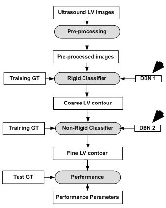Figure 8

DBN based LV contour tracking model.

Figure 9

Output of DBN-based segmentation of LV. The auto detected outline is shown in yellow, COM (40) outline in magenta, MMDA (41) outline in cyan while the GT outline is shown in blue (reproduced with permission from (39)).

4.1.2. Fully automatic segmentation of the left ventricle in cardiac MRI

Automated LV segmentation using conventional methods suffers from primarily two issues. The first is the lack of large training data and the second there is shortcomings in classical deformable models i.e., leakage, shrinkage and sensitivity to initialization. The combined approaches of DL along with deformable models can be used to resolve limited data size issue and the shortcomings of classical deformable models using artificial data enlargement, pre-training and careful design. In here an integrated approach of DL and deformable models in segmentation and alignment of the left ventricle (LV) from cardiac magnetic resonance imaging (MRI) datasets (43).

The MRI were obtained from 45 cardiac MR Datasets taken from the MICCAI 2009 LV segmentation problem. At first, the MRI were the input into the CNN framework to obtain the binary masks. The binary masks were then used to generate the region of interest (ROI) from the MR images. The weights of the CNN framework itself were next trained by an autoencoder. Once the ROI was obtained, an initial LV shape $δ^{(0)}$ was inferred from the ROI using stacked autoencoder architecture. Deformable models were applied in the final stage for segmenting the LV and final 3D alignment from the inferred shape. This was done by minimizing the energy function over the inferred shape which is given by:

δ = \arg \min_{δ} E (δ)

$δ^{(0)}$ denotes the optimal contour shape. This was done by updating initial shape $δ^{(0)}$ iteratively using gradient descent method to obtain the final contour which is given by:

$δ^{(i + 1)} = δ^{(i)} + γ \frac{d δ}{d t}$ (11)

where $γ$ denotes the step size, i represents successive iterations and $\frac{d δ}{d t}$ represents change in $δ$ with respect to time. The model with respect to the system is given in Figure 10. The 2D and 3D segmentation outputs are shown in Figure 11 (a) and Figure 11 (b). Dice metric (DM), average perpendicular distance (APD) and conformity metrics were computed from the output estimated and GT contours. The results have shown improvement over previous methodologies with DM at 0.94, APDat 1.81 mm and conformity at 0.86.

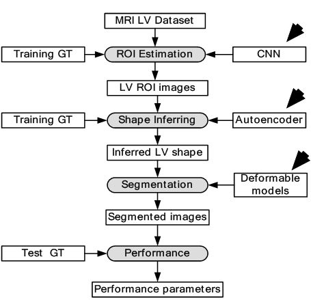Figure 10

DL-based LV contour tracking model for MRI.

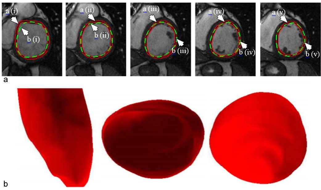Figure 11

(a). Example of outputs from the DL-based LV segmentation. The auto detected LV contour is shown in red-black as pointed by arrow (a) while GT contour is shown in green as pointed by arrow (b) (reproduced with permission from (42)). (b). Inferred 3D shape from the given model with side, top and bottom cut-sections (reproduced with permission from (42)).

Although the model gives a quicker convergence with respect to classical methods, it is not fast enough since it is a CPU-based framework. All current versions of DL are GPU-based and therefore give a faster convergence rate. The CNN and autoencoder architectures implemented in this paper are one layer deep. However, all current DL frameworks are deeper i.e., multiple layers. Therefore, there is a scope of improvement by increasing the number of layers and be called truly deep. Even if the performance parameters are better than classical methods, the system can be improved for clinical acceptance.

4.1.3. Volumetric left ventricle image parsing

The success or failure of ML-based algorithms lies with the human understanding of prior information hidden in the data to design feature extraction methods. This feature extraction task becomes even more complex in case of volumetric or 3D data. This is because the system tries to capture features/parameters in translation (3D), orientation (3D) and anisotropic scale (3D) of the desired object, resulting in finding features in 9D space. Such large number of parameters scanning is not possible with current systems. A novel idea of Marginal Space Deep Learning (MSDL) (44) was introduced where incrementally learning deep classifiers are employed to learn the location of LV in the 3D image. This method was applied in two stages: a) object localization and b) boundary estimation. The object localization is done by applying deep classifiers (DCs) stepwise to learn position-orientation-scale of the LV. It is done by maximizing posterior probability of location of the object in image I which can be defined as:

$(\vec{T}, \vec{R}, \vec{S}) = \arg \max_{\vec{T}, \vec{R}, \vec{S}} (\vec{T}, \vec{R}, \vec{S} | I)$ (12)

where $\vec{T}$ represents the 3D translation, $\vec{R}$ denotes the 3D orientation and $\vec{S}$ signifies the 3D scale space. The DC applied in this paper is Fully Connected Network. As observed in Eq. 14, a rough estimate is made on the position, orientation and scale of LV by using three DCs. The first DC is used to estimate the position of LV using 3D translation. By using the position estimate of the first DC, the second DC is used to estimate the position and orientation of LV. At last, by taking into account the position and orientation estimate from the second DC, the third DC estimates the position, orientation and scale of the LV. In the border estimation stage, DL-based active shape model is applied to guide the shape deformation. In order to increase computational efficiency and prevent overfitting, sparsity is introduced into the network by gradually dropping neural connections without affecting network performance. The dataset is taken from 869 patients containing 2,891 3D volumes from different vendors. The results have shown considerable improvement over state of the art Marginal Space Learning (MSL). The MSDL position error is computed at 1.47 mm which is far lower compared to 3.12 mm in MSL. The MSDL corner error is found to be 2.80 mm which is almost half the corner error of 5.42 mm in MSL. The corresponding model is given in Figure 12.

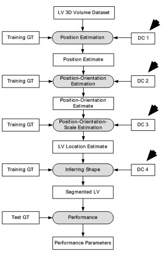Figure 12

Deep classifier-based 3D LV segmentation model.

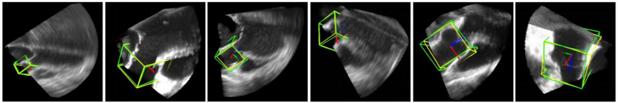Figure 13

Deep Classifier-based 3D LV segmentation model outputs. The auto detected bounding box is shown in green while the GT bounding box is shown in yellow (reproduced with permission from (43)).

The resultant images are shown in Figure 13. The results provided in this study are not sufficient to judge the efficiency of the scheme. However, this method is the first application of DL in 3D imaging and therefore can be considered a benchmark in volumetric image parsing.

4.1.4. Vessel extraction in X-Ray angiograms

Coronary artery disease (CAD) is the most common type of heart disease which is the leading cause of death globally. X-ray angiography is considered as important method for diagnosis of CAD. Tracking and filter based methods for vessel extraction suffers from non-linear noise, multiple organ structures bringing complexity in the images, and lastly low resolution. In study (45), a DL-based approach using CNN is proposed for detecting vessel regions in angiography images. A dataset of 44 X-ray angiography images is considered for the experiment. All the images were manually segmented by an expert. The images were first pre-processed to increase the contrast by Top-Hat transform. In order to train the CNN, 1,040,000 patches were extracted and applied. The patch is defined by placing a window around each pixel of the image. Each patch is fed into the CNN for training/testing. The CNN consists of two convolutions, two max-pooling and two FC layers. The first fully connected layer consisted of 500 neurons and the second consisted of two neurons. The two neurons generated two probabilities for the center of the patch if it either belonged to the vessel region or the background region. The test results showed an accuracy of 93.5%.The whole object process model is shown in Figure 14. The DL-based method showed greater accuracy values in spite of low resolution and complex background of the images which demonstrated its superiority over conventional models. However, deeper architectures are needed to be tried for optimal results. A comparative analysis with current medical techniques for diagnosis is required to judge its clinical efficacy. The segmentation outputs are shown in Figure 15.

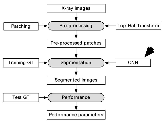Figure 14

Segmentation of X-ray images using CNNs.

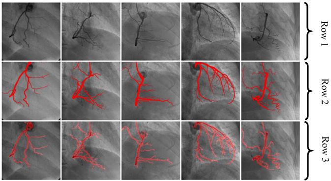Figure 15

Row one shows five input images. Row two shows corresponding GT of Row one images. Segmentation outputs analogous images using CNN shown in row three (reproduced with permission from (44)).

4.1.5. Plaque characterization

An important task for identifying cardiovascular disease (CVD) events is the identification of plaques that are prone to rupture. Identification of such plaques is important for early risk assessment of cardiovascular and cerebrovascular events. The significant US speckle noise, coupled with the small size of the plaques and their complex multifocal appearance, makes it difficult even for automated ML techniques to discriminate between the different plaque constituents. Also, the US images of carotid bifurcation are inundated by shadowing, artifacts and reverberation making them difficult to read even by experts. This motivated Karim et al. (46) to implement automatic plaque characterization using DL-based framework. The study applied CNN-based strategy for plaque characterization. The CNN consisted of four convolution layers followed by three fully connected layers. Each of these layers was followed by a ReLu layer for extraction of deep features. A fully connected layer and softmax layer were appended for characterization purpose. The cross-entropy loss function was used for training. The cross-entropy describes the loss between two probability distributions. In the case of DL, it describes the loss between true and predicted probability distribution. Single-scale SVM and multi-scale SVM was used for benchmarking the results of DL-based system.

The study considered 90,000 image patches that were extracted from 56 US CCA images. All the patches were annotated into three classes of plaque such as: lipid core, fibrous and calcified by a single expert clinician with decades of experience. The annotated patches formed the GT of the experiment. The corresponding model of the system is shown in Figure 16. Finally, predicted plaque labels were compared against GT for performance parameters. The characterization results are shown in Figure 17. The DL-based approach gave the best classification accuracy at 78.5% of the cases, while multi-scale SVM gave classification accuracy of 14.3% and single-scale SVM gave classification accuracy of 7.2%.

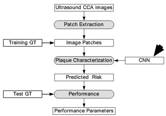Figure 16

Global diagram for plaque characterization.

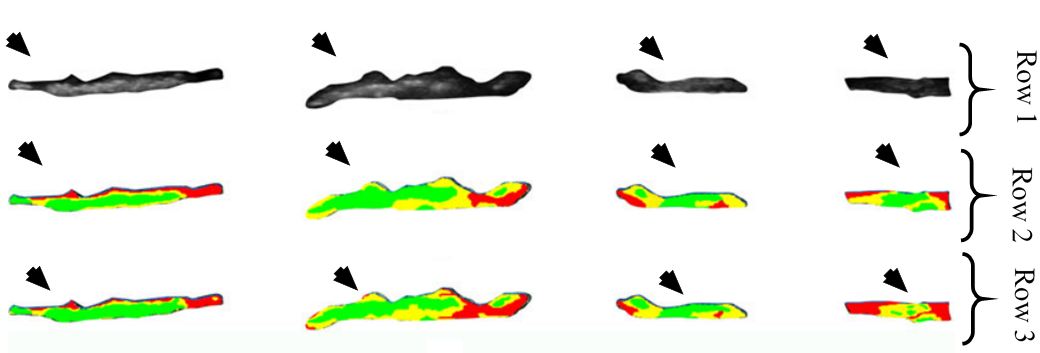Figure 17

Row one represents input images, row two is the corresponding GT and row three is the equivalent characterization output of the given method. In here, red represents lipid core, yellow epitomises fibrous tissue and green signifies calcified tissue (reproduced with permission from (45)).

The author has presented a useful DL system for plaque characterization using deep features for characterization by SVM based classifiers. The dataset size for the experiment was limited to 56 images only and hence more data set was needed to prove its validity and robustness. The classification accuracy was low when compared against other medical CAD systems.

4.2. Neurology application

Identification of abnormal regions of brain is a challenging task due to mixture of intensities in the images and irregularities of the abnormality. In here we discuss some applications of DL in neurology.

4.2.1. Brain lesion segmentation

In brain imaging, exact estimation of location of lesion from traumatic brain injury (TBI) pertinent to brain structure is a necessity. There are several complications in computational estimation of brain lesion i.e., they can occur at multiple sites, shape and size of lesions vary and their intensity profiles overlap with healthy parts of the brain. Several conventional methods have been developed to localize 3D brain lesions but their performance is limited. This motivated the development of DL-based architecture for brain lesion segmentation (47). In this review, two DL-based architectures were used in parallel to increase the accuracy of estimation. Each DL-based pathway is a CNN which processes a different scale of the input which are combined to give accurate segmentation of brain lesion. In the first pathway, original size 3D images were input into the system whereas in the second pathway downsampled 3D images were fed. The first pathway computes the detailed local appearance of the structure while the second pathway captures high level features such as location within the brain. The features from these two pathways are combined later. The second pathway features are upsampled and then combined with the first pathway features. Finally, the combined 3D features are fed into 3D fully connected conditional random field (CRF) network for structural predictions. The data were collected from 66 patients with moderate to severe traumatic brain injuries. The method gave highest dice similarity coefficient (DSC) at 0.59 at the ISLES-SISS challenge 2015. The corresponding model is given in Figure 18. The segmentation outputs of the model is given in Figure 19. The results were compared against the Random forest method and the DL-based method outperformed the Random forest methodology. However, the DSC values are low making the methodology questionable for clinical use. However, this model provides prototype for DL-based frameworks for brain lesion segmentation.

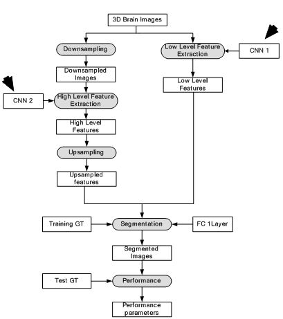Figure 18

Deep Neural Network for brain lesion segmentation.

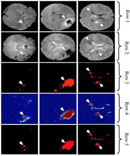Figure 19

Row one and two represents the FLAIR and DWI sequences from the dataset, row three denotes the GT, row four shows the corresponding output of DeepMedic and row five shows the analogous output of DeepMedic + CRF (reproduced with permission from (46)).

4.2.2. Brain tumor segmentation

Among several types of brain tumor, Gliomas have the highest mortality rate. Gliomas are divided into two types: low grade gliomas (LGG) and high grade gliomas (HGG) with the latter being more aggressive than the former. Segmentation of Gliomas and their characterization into LGG and HGG is important for treatment, planning, and follow-up evaluation of the patients. Manual segmentation of Gliomas is tedious and error prone and therefore requires semi-automatic and automatic methods for segmentation. The detection of Gliomas is difficult because of their variable shape, structure and location. The MRI present their own set of challenges in form of intensity homogeneity and different intensity ranges along the same sequence of images and faulty acquisition scanners. Conventional methods such as ML-based techniques have been applied for segmentation but with limited success because of the above mentioned challenges. DL methods that generate their own internal features stand as an interesting alternative to the conventional methods. In this paper (48), a CNN architecture has been applied for tumor segmentation. The tumors are divided into four classes such as: edema, necrosis, non-enhancing and enhancing. The images were pre-processed before they are input into the DL system for training. The pre-processing involved normalization of the image dataset.

Two different CNNs of different depth were used for LGG and HGG. The depth of LGG CNN was lesser compared to HGG CNN as increasing depth for LGG CNN did not increase performance. The LGG CNN framework consisted of four convolutions, two max-pooling and three fully connected layers while the HGG CNN framework consisted of six convolutions, two max-pooling and three fully connected layers. Two kinds of datasets were used for the experiment such as: BRATS2013 and BRATS2015. BRATS2013 contained 65 MRI scans and BRATS2015 consisted of 274 MR scans with manual segmentation available for both. For training, 335,000 and 450,000 image patches were extracted for LGG and HGG images respectively. The dice similarity metric for complete, core and enhancing segmentation scheme was 0.88, 0.83 and 0.77 respectively. The object process diagram is shown in Figure 20. Since only 339 images were used, there is a scope of better training of the CNN with larger dataset. The segmentation output images are given in Figure 21. There is a clear potential of improvement of performance.

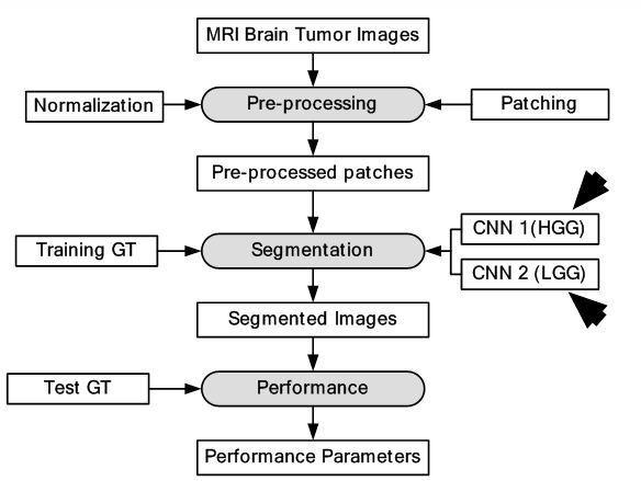Figure 20

DL-based system for brain tumor segmentation.

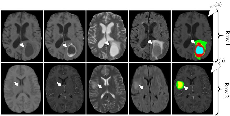Figure 21

Segmentation of HGG shown in row one and segmentation of LGG shown in row two. The different MRI sequences from left to right are T1, T1c, T2 and FLAIR. The rightmost image in row one shown by medical arrow (a) is HGG segmented image and rightmost image in row two shown by medical arrow (b) is LGG segmented image. The colors represent tumor types: green: edema, blue: necrosis, yellow: non-enhancing tumor and red: enhancing tumor (reproduced with permission from (47)).

4.3. Mammography application

Breast cancer diagnosis provides various challenges to medical imaging scientists. Below, we discuss some applications of DL to detect breast cancer cells in breast cancer images.

4.3.1. Mitosis detection in breast cancer

The presence of mitotic figures in histology images is an important indicator of cancer. Mitosis is a complex process where the cell nucleus undergoes various transformations. There are several structures of same intensity and shape that appear in histology images out of which only few are mitotic cells. Therefore, identification of mitotic cells becomes a difficult task. In this study, each pixel is assigned two classes which are: mitosis and non-mitosis. DL was applied for classification of pixels in the given dataset (49). Two different CNN frameworks were trained. The first CNN was 13-layer architecture and consisted of input, five convolutions, five max-pooling and two fully connected layers. The second CNN was 11 layers with one input, four convolutions, four max-pooling and two fully connected layers. The final outputs were later combined in ensemble classifier. A total of 50 images were taken from public MITOS dataset for training and testing of the DL-based pixel classifier. The performance results of our DL-based approach showed a precision of 0.88 and F1-score of 0.78 which is higher than all previous implementations. The object process model is shown in Figure 22. The characterization output is presented in Figure 23.

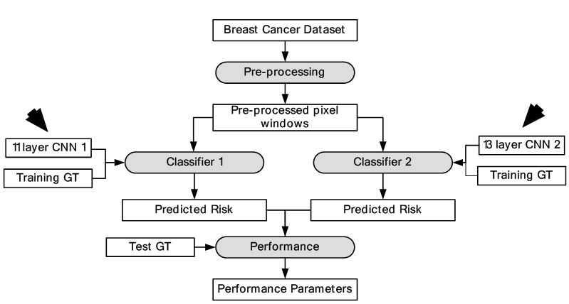Figure 22

DL-based breast cancer detection.

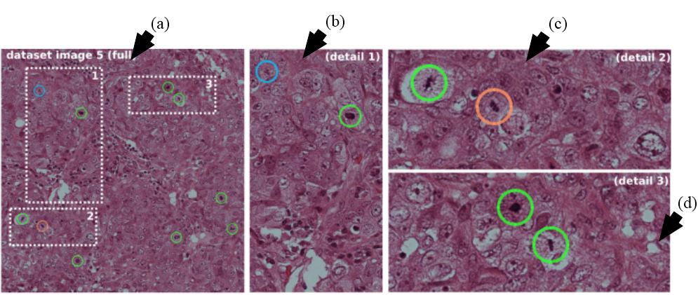Figure 23

Leftmost image show by arrow (a) represents the image with three dotted areas. The three dotted areas are shown in detail as pointed by arrow (b), arrow (c) and arrow (d). Mitosis detected by the system shown in green, red represents false positive and cyan signifies mitosis not detected by the given approach (reproduced with permission from (48)).

The size of the dataset was limited to 50 images. Although the method gave the best accuracy in comparison with competitors at ICPR2012 (48), the method requires a larger data size and corresponding validation.

4.3.2. Digital mammographic tumor classification

Computer aided diagnosis of breast cancer using ML involves extraction of features and estimating malignancy probabilities. The methodology focuses on classification of breast lesions from mammographic images using transfer learning via CNN framework (50). In this study, classification comparison was made between analytically extracted hand crafted lesion features and features obtained from deep CNN. The deep CNN was trained on general object recognition tasks different from the breast cancer data through a process known as transfer learning. It is based on the hypothesis that structures within a CNN trained on everyday objects can be used to create a classifier for breast cancer. The dataset consisted of 219 breast lesions on digital mammography images from which 607 region of interests (ROIs) were extracted. AlexNet - a CNN model was selected for feature extraction from breast cancer dataset. It consists of three fully connected layers and five convolutional layers. Three of the five convolutional layers were followed by max-pooling layers. Two SVM classifiers, were used for training and testing of features obtained from AlexNet (Method A) and analytically extracted lesion features (Method B). An ensemble technique called soft voting was used to combine the results of two classifiers, which is if p1 was output of Method A and p2 was output of Method B, then the output of ensemble classifier was (p1+p2)/2. It’s seen from the results that ensemble classifier was significantly better i.e., AUC was 0.86 than Method B, that is, SVM trained on analytically extracted features i.e., AUC was 0.81. The analogous model is given in Figure 24. The outputs of each layer are shown in Figure 25. The study provided important benchmarking results in terms of AUC, but the system did not use GPU-based paradigm.

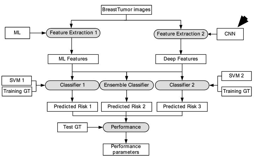Figure 24

DL-based breast tumor detection.

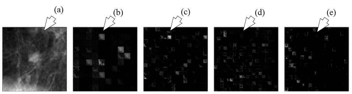Figure 25

The outputs of different layers of AlexNet are shown. (a) represents the ROI input, (b) represents output of pooling layer one, (c) denotes outputs of pooling layer two, (d) denotes output of convolution layer four and (e) signifies the output of pooling layer five which are fed into conventional methods for characterization (reproduced with permission from (49)).

4.4. Microscopy application

Biological cell identification from images is a very difficult and time consuming task. In here we discuss some applications of DL in microscopy.

4.4.1. Quantitative analysis of individual cells in live-cell imaging experiment

In the field of cellular biology, dynamic live-cell imaging experiments are a powerful tool to interrogate biological systems. Determining the class of cells requires hours of manual curation. The key to analyzing data generated by these measurements is image segmentation i.e. identifying which parts of an image (pixel) belong to which individual cells. The conventional methods applied to microscopic cell segmentation still require substantial manual curation for segmentation accuracy. DL-based methods provide an alternate way to improve segmentation accuracy as DL frameworks generate features internally. The DL framework implemented here was CNN architecture (51). By integrating CNNs into an image analysis pipeline, one can quantify the growth of thousands of bacterial cells and track individual mammalian nuclei with almost no manual correction. The training dataset is created from images of representative class by taking each image pixel and annotating a small region (patches) around a pixel with the pixel’s respective class. This is done for all images in the dataset. The image segmentation becomes a classification task as now the segmentation involves splitting images into overlapping patches, by applying classifier to each patch to assign labels and then all labels are congregated to form a new image. This prediction image is converted into segmentation mask by using image processing techniques. The cost function applied here is given by:

$c = - \sum_{i} \log (\frac{e^{l a b e l}}{\sum_{l} e^{i}}) + τ \sum_{w \in W} w^{2}$ (13)

where C represents the cost function, i symbolizes the images, l denotes the labels, w signifies weights, $τ$ corresponds to regularization parameter and W signifies all weights. The weights are updated as per the given formula:

$w_{i + 1} = w_{i} - γ \frac{\partial C}{\partial w}$ (14)

where i denotes iterations, $γ$ represents the learning rate and $\frac{\partial C}{\partial w}$ gradient of cost with respect to weight.

A total of five different mammalian cell lines were used to create the annotated dataset. In one microscopic image, the number of bacteria cells were approximately 300, 500 nuclei and 100 mammalian cells. The image dataset was first normalized for increasing robustness, segmentation performance, and processing speed and then augmented by rotating each image patch by 0, 90, 180, or 270 degrees. It was done to make the class labels invariant to the transformations. In order to generate a prediction for each pixel, a trained FCN was applied for segmentation. The jaccard index (JI) and DM for mammalian nuclei were 0.89 and 0.94 respectively. Model parallelism was used to increase segmentation accuracy. The corresponding model is shown in Figure 26. The output is given by Figure 27. The application of DL-based framework reduced human curation time significantly and improved the accuracy of segmentation mask. The CNN architecture details which are not present would have provided more insight into the depth of the network.

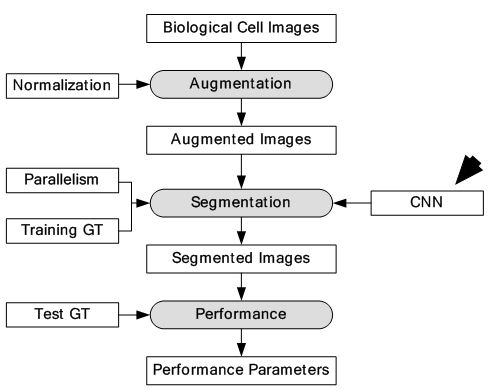Figure 26

Model depicting segmentation of individual cells using DL.

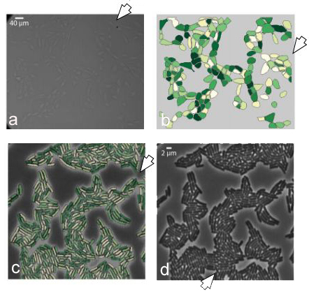Figure 27

The phase contrast input images are shown leftmost side and pointed by (a) and (d). The analogous segmentation output is shown (b) and (c) (reproduced with permission from (50)).

4.4.2 Classifying and segmenting microscopy images

The high-content screening (HCS) technologies have enabled large scale imaging experiments for studying cell biology and for drug screening. The ML-based algorithms available are optimized for mammalian cells and not for tiny organisms such as yeast. The DL approaches that learn feature representations directly from pixel intensity values have currently dominated object recognition challenges worldwide. In this study, the approach has been to combine CNN with multi-instance learning (MIL) in order to segment microscopy images using only whole image level annotations (52). In MIL, the supervised algorithm trains not from single instances rather a group of instances at a time. The similarity between the pooling layer and the MIL aggregation function is exploited here, where features in convolutional layers correspond to instance features in MIL. If class specific feature maps are treated as bags of instances, then the classical approaches in MIL can be generalized to global pooling layers over these feature maps. The CNN produces an image level classification over images of arbitrary size and varying number of cells through a MIL pooling layer. The individual cells are classified by mapping the probabilities in class specific feature maps back to the input space. The pre-softmax activations of specific output nodes are back-propagated through a classification network to generate Jacobian maps with respect to specific class predictions. The segmentation masks are generated by thresholding the sum of the Jacobian maps along the input channels. Loopy belief propagation (reference #10 in (52)) is used to improve the localization of cellular images with respect to segmentation masks. The DL framework consisted of seven convolution layers, four pooling layers, one MIL pooling layer and one fully connected layer. A total of three types of datasets were used. Data was collected from nine categories of MNIST handwritten digits dataset. From each category, 50 images were used for training and 10 images were used for testing. The second dataset consisted of MFC-7 breast cancer cells available from the Broad Bioimage Benchmark Collection. A total of 300 microscopic images were used for training and 40 images were used for testing. Cell data was also collected from yeast GFP collection. A total of 2200 images were used for training and 280 images were used for testing. The equivalent model is given in Figure 28. The segmentation is output is shown in Figure 29. The test error for MNIST dataset was 0%. The highest accuracy for yeast dataset and breast cancer dataset across all classes was 0.96 and 0.97 respectively. The results showed considerable increase in accuracy across all datasets. The system should be validated with larger breast cancer dataset to increase its clinical value.

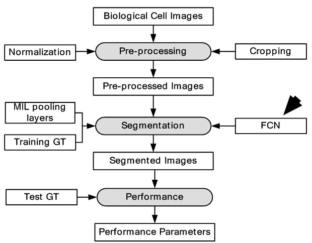Figure 28

Model depiction deep multiple instance learning.

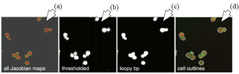Figure 29

Segmentation using FCN-MIL pooling methodology. (a) Shows the Jacobian maps, (b) shows thresholding, (c) denoising using loopy bp and (d) segmentation outlines (reproduced with permission from (51)).

Recently, DL has also been applied to enhance super-resolution localization microscopy (53), Resolution enhancement of wide-field interferometric microscopy (54) and rapid autofocusing in whole slide imaging (55).

4.5. Dermatology application

Skin cancer affects a considerable percentage of population across the globe. In here we discuss one application of DL in characterizing skin cancer from images.

4.5.1. Melanoma recognition in dermoscopy images

Melanoma has the highest mortality rate among skin cancers. It is curable when detected at initial stage. The ML algorithms applied earlier for detection of melanoma are dependent on hand-coded low-level features and therefore their success was limited. In this study, DL was applied for detection of melanoma (56). The segmentation was done by an FCN whose architecture was similar to UNet (57). It co4nsisted of a series of convolutions, pooling followed by a single fully connected layer. It was followed a series of deconvolution and unpooling layers. Skip connections were used to merge convolutional data prior to pooling operations with the deconvolution operation outputs. The classification operation consisted integration of CNN, DRN and UNet. Each technique is used to extract features from the entire image and region segmented around the lesion part. The architecture consisted of three stages of convolutions and pooling followed by fully connected layer and thereby the process is reversed with three stages of deconvolution and unpooling layers. For this experiment, 900 annotated dermoscopic images were used for training and 379 images were used for testing. The dataset was a part of the ISIC2016 (reference #34 in (56)). The proposed system consists of two primary components: segmentation and classification. At the end, an SVM was applied to segregate the melanoma. The system gave higher accuracy at 76.0% in comparison with 70.5% of average accuracy of eight dermatologists. The whole object process model is depicted in Figure 30. The segmentation output is shown in Figure 31.

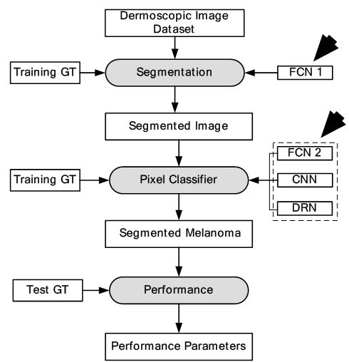Figure 30

Segmentation and classification of melanoma.

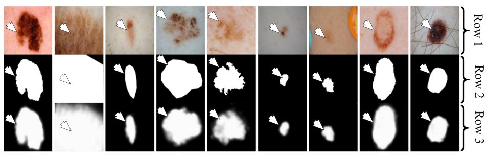Figure 31

Segmentation of melanoma of nine patients using FCN-UNet. Row one shows the input images. Row two is the corresponding GT and row three is the analogous segmentation output (reproduced with permission from (52)).

Although the results are better than eight dermatologists, the system did not meet the accuracy standard for regulatory level.

4.6. Gastroenterology application

Liver tumor detection is a challenging task. In here, we discuss one application of segmentation of liver tumor from CT images.

4.6.1. Segmentation of liver tumor

As per WHO report, liver cancer has been the second major cause of death among all cancers. Detection of liver tumor from CT images is tough task appearance variability, fuzzy boundaries and heterogeneous densities, shapes and sizes of lesions. Earlier applications of ML had limited performance due to their dependence on hand-made feature extraction algorithms. In here (58), DL-based framework has been used for segmentation for liver tumor.

A CNN architecture is used as the DL-based framework. The CNN consisted of two convolutions, two max-pooling, one fully connected and one Softmax layer. Three ML algorithms which are AdaBoost, Random Forest (RF) and SVM were used for benchmarking the results. The images were pre-processed and patches were extracted from the images. Each patch was labelled positive if more than 50% of it contained tumor cells and negative otherwise. All the patches were fed into the CNN for training and testing. A dataset of 30 CT images was collected for the experiment. The CT images were divided into two categories of tumor and non-tumor images. The comparison results show DM coefficient at 80.06% for the given method, 79.78% for SVM, 79.47% for RF and 75.67% for AdaBoost. The segmentation system model is visualised in Figure 32. The segmentation output is given in Figure 33. The results have shown considerable improvement over ML based techniques, however, there was a clear potential of improvement in terms of accuracy.

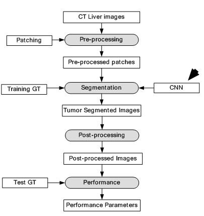Figure 32

Segmentation of CT liver tumor.

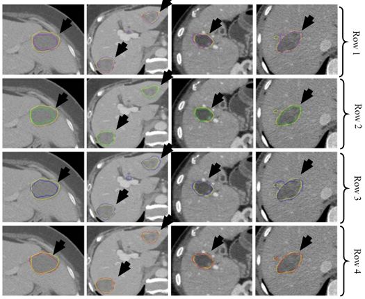Figure 33

Segmentation of CT liver tumor for four patients using AdaBoost (purple) in row one, RF (green) in row two, SVM (blue) in row three and CNN (red) in row four. GT is shown in yellow in all rows (reproduced with permission from (54)).

4.7. Pulmonary application

Detection of lung cancer using automated techniques is always a challenge. In here we discuss one application of DL in lung cancer characterization from images.

4.7.1. Characterization of lung disease

Lung cancer is a malignant disease with five year survival rate less than 20%, if not diagnosed early. Characterization of lung disease from CT images is difficult as small lung nodules are infrequently regarded malignant, difficult to biopsy and cannot be reliably characterized by positron emission tomography scan. DL-frameworks provided a new area of research in this field. In here for characterization of lung cancer (59), two DL-based frameworks are applied. Two separate characterizations were done using two DL techniques such as: CNN and DBN. It was found that CNN and DBN both gave better results than other conventional methods using feature extraction technologies. The pulmonary modules in lung could be diagnosed as malignant based on their shape which can be sphericity and speculation and composition of internal structures such as fluid, calcification and fat. In this paper, the chest CT images were collected from 1010 patients. The sensitivity of CNN and DBN was found to be 73.3% and 73.4% while specificity was found to be at 78.7% and 82.2%. The object process model of the system is given in Figure 34. The input CT images depicting various sizes of lung module is given in Figure 35. This application can be called as a ground level study of the use of DL for lung cancer detection. Multiple deeper layers could be added to improve accuracy. The paper lacked prevailing DL-based architectures.

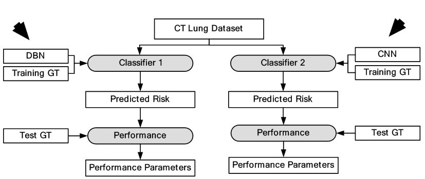Figure 34

Characterization of CT lung cancer.

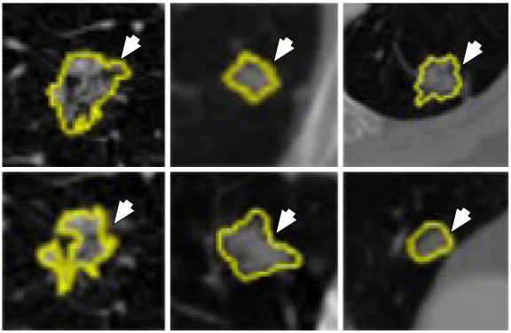Figure 35

Different sizes of lung nodules (yellow) visualized in the CT images for characterization by the CNN and DBN (reproduced with permission from (55)).

5. DISCUSSION

The evolution of DL can be traced to earlier attempts to mine knowledge using artificial intelligence (AI) techniques from given data. The AI techniques were task specific and faced difficulties dealing with real time data. This led to the development of ML which was able to learn patterns from data using feature extraction tools. The ML techniques were dependent on feature extraction techniques which were faulty in nature. The feature extraction methodologies are generally hand-designed mathematical tools and therefore task specific. These tools cannot be diversified to the wide variety of real time data that exists. Therefore, the performance of ML system is limited. The advantage of DL is that it generates its own features and is independent of feature extraction techniques. Thus, the performance of DL system is better than ML systems. The greater depth of DL system allows it to learn complex functions and composite relationships between data components. The application of DL system varies widely i.e., text, numbers, images, video etc. In this paper, our primary focus has been on DL in medical imaging applications. We have dealt with various types of images like US, MRI, CT, X-ray etc. from various types of medical fields i.e., cardio, neurology, mammography, microscopy, dermatology, gastroenterology and lung as seen in Table 1. The DL system deals with characterization and segmentation. The characterization is done in one stage by classifying images as per the labels which is followed in rows 5, 8, 9 and 14. We have observed two kinds of segmentation. In general segmentation in ML system follows the active contour models (60). The first kind is a two-stage system where a rough estimate is made about the contour in the first stage and in the then fine tuning is done in the second stage for fine segmentation. This type of segmentation is followed in rows 1, 2, 3, 6 and 11. The first stage is usually a DL framework but the second stage is implemented by either DL or conventional methods. In the second kind, segmentation is performed in first stage itself. There are again two ways to do that. The image is divided into very small patches, and each patch is classified as per the labels. These labels are reassembled to give the segmentation mask of the given image. This way of patching, classifying and reassembling can be seen in rows 4, 7, 10 and 13. The second way is semantic segmentation using FCN which is observed in row 12. In addition to mentioned research, DL has also been applied recently in brain lacunes detection (61), white matter segmentation (62) and fatty liver disease detection (63), which are not discussed due to lack of space. Generalized DL systems which can do classification, regression and segmentation for wide variety of medical images has also been developed (64). It was observed that despite the wide diversity of image and application types, DL systems were able to give higher performance, greater accuracy and lower error. This proves that the robustness and performance of DL systems are independent from diversity and origin of data. In the next subsections, we discuss the hardware and software requirements for DL.

Table 1.Benchmarking table

Medical field	SN	Author (year)/Ref number	Data type (size)	Application type	DL System (Stage 1)	DL System (Stage 2)	Performance
Cardiovascular	1	Gustavo et al. (2013) [40]	US (496)	LV Segmentation	DBN	DBN	JD: 0.83, AV: 0.91, MAD: 0.95, AVP: 0.83
	2	Avendi et al. (2008) [43]	MRI (45)	LV Segmentation	CNN	Autoencoder + Deformable model	DM: 0.94 ±0.02, APD: 1.81 ±0.02 mm, Conformity: 0.86
	3	Ghesu et al. (2016) [44]	3D TEE (2891)	LV Segmentation	Fully Connected Network	Fully Connected Network	Position Err: 1.47 mm Corner Err: 2.80 mm
	4	Esfahani et al. (2016) [45]	X-ray (44)	Vessel Segmentation	CNN	-	Acc: 93.5 %
	5	Karim et al. (2017) [46]	US (56)	Plaque Classification	CNN	-	Acc: 0.75 ±0.16
Neurology	6	Kamnitsas et al (2017) .[47]	3D TBI (66)	Brain lesion Segmentation	CNN	Fully Connected Network	DM: 0.59
Neurology	7	Pereira et al (2016) .[48]	MRI (339)	Brain tumor Segmentation	CNN1 (HGG) + CNN2 (LGG)	-	DM complete: 0.88 DM core: 0.83 DM enhancing: 0.77
Mammography	8	Ciresan et al. (2013) [49]	MITOS (50)	Mitosis Classification	CNN1 (11 layers) + CNN2 (13 layers)	-	Precision: 0.88 F1-score: 0.78
Mammography	9	Huynh et al. (2016) [50]	Dig. Mam. (219)	Breast tumor Classification	CNN + SVM	-	AUC: 0.86
Microscopy	10	Valen et al. (2016) [51]	Mammalian cell lines (5)	Cellular Segmentation	CNN	-	JI (MN): 0.89 DM (MN): 0.95
Microscopy	11	Kraus et al. (2016) [52]	Breast cancer (340) Yeast (2480)	Cellular Segmentation	CNN+MIL	Jacobian Maps + loopy belief propagation	Breast cancer Acc: 0.971 Yeast dataset Acc: 0.963
Dermatology	12	Codella et al (2016) . [56]	Dermatology (1279)	Melanoma Segmentation	FCN	-	Acc: 76%
Gastroenterology	13	Li et al. (2015) [58]	CT (30)	Liver tumor Segmentation	CNN	-	DM: 80.06%
Pulmonary	14	Hua et al. (2015) [59]	CT (1010)	Lung Cancer Classification	CNN DBN	-	CNN Sens: 73.3 % DBN Sens: 73.4 %
JD: Jaccard Distance; AV: Average Error; MAD: Mean Absolute Distance; AVP: Average Perpendicular Distance; DM: Dice Metric; APD: Average Perpendicular Distance; TEE: transesophageal echocardiogram; TBI: Traumatic brain injury; JI: Jaccard index; MN: Mammalian nuclei

5.1. Graphics Processioning Unit

Deep neural networks need to learn millions of weights while training. However, training such huge number of weights on a single, dual and even seven core CPUs may take weeks to complete. A graphics processing unit (GPU) consists of hundreds of cores and a peak memory bandwidth several times higher than a normal CPU, makes it an attractive option for DL. The computer hardware operates thousands of threads and can schedule them on the available GPU cores thus offering massive parallelism over CPU operations. Thus, the speedup of GPU is almost 10 to 100 times of a CPU based core, therefore, completing jobs in few hours. However, the massive speedup requires dedicating cores for data processing rather than caching and control like a normal CPU core. Therefore, algorithms for ML should be rewritten for running on GPU. In spite of the disadvantage of using GPU, CPU is still not practical for their low speed (8).

5.2. Software Frameworks for DL

The complexity of DL systems requires suitable software framework for its implementation. Python is the most popular programming used for DL applications. It provides unique set of easy to use library functions for implementation of DL architecture. Most of the software frameworks discussed in this subsection are partly or fully developed in Python language. The most popular among them are TensorFlow (65), Theano (66), Keras (67), CAFFE (68), Torch (69) and Deeplearning4j (70). TensorFlow is a second-generation DL system developed by the Google Brain team. TensorFlow is a Python-based library capable of running on multiple CPUs and GPUs. Theano like TensorFlow is Python-based low-level library for developing DL applications. However, unlike TensorFlow it lacks multiple-GPU support. Keras as an interface built to work on either Theano or TensorFlow. It is also developed in python and requires fewer lines of code to build a DL system. CAFFE is a C++ library with both Python and MatLab interface. The primary application of CAFFE is in developing CNNs. It is open sourced by Facebook as a simpler version in the form of Caffe2. Torch is a C/C++ library and CUDA for GPU processing. Torch was built with an aim to achieve maximum flexibility and building of models extremely simple. It is now also available in Python in the form of PyTorch. Torch is a C/C++ library and CUDA for GPU processing. It is now also available in Python in the form of PyTorch. Deeplearning4jis Java based toolkit and supports JVM. It can be implemented on top of the popular Big Data tools such as Apache Hadoop and Apache Spark. It is widely used as a commercial, industry-focused distributed DL platform.

Though the discussion has been strictly focused in medical imaging, the DL usage and applications are wide-ranging in healthcare. DL has been successfully applied in genomics and biomedical signal processing. In genomics, DL has been successfully applied in protein structure prediction (71-79), gene expression regulation (80-84), protein classification (85-87) and anomaly classification (88). In biomedical signal processing, DL has been applied to brain decoding (89-91) and anomaly classification (92-94). The only reason for applications of DL in wide areas in a very short span of time, is its independence from different feature extraction methodologies. The high performance of DL systems underlines quick diagnosis of disease and even better monitoring of high risk patients. Therefore, patient treatment can start quicker and help in quick recovery of the patients leading to a better healthcare ecosystem.

6. CONCLUSION

In this paper we have focused on 14 papers of deep learning in various medical imaging applications such as ultrasound, MRI, CT-scanned images etc. from various domains such as cardio, neurology, mammography, microscopy, dermatology, gastroenterology and pulmonary. It’s been seen that DL-based applications give far better accuracy than conventional methods. This due to their in-house feature extraction capability which increases their accuracy. The main focus of this review has been on classification and segmentation. For each DL application object process model has been drawn which shows us the inner working of the DL-based systems. In the future, we would evaluate real time medical imaging applications of deep learning and develop a future model for real time applications.

7. ACKNOWLEDGEMENT

We would like to thank the publishers for approving usage of images in our paper. We would like to thank MediaLab Asia, DEITY for their encouragement and support.

References

[1]

LeCun

, Bengio

and Hinton

Deep learning. Nature, 521436444 2006https://doi.org/10.1038/nature14539PMid:26017442