


 , Xiaoou Li 2, Shouwei Gao 1, Peng Zan 1,*,†
1 School of Mechatronic Engineering and Automation, School of Medicine, Research Center of Brain Computer Engineering, 200444 Shanghai, China
2 School of Medical Instrument, Shanghai University of Medicine & Health Science, 201318 Shanghai, China
3 Engineering Research Center of Traditional Chinese Medicine Intelligent Rehabilitation, 200444 Shanghai, China
†These authors contributed equally.
Abstract
Background: The adoption of convolutional neural networks (CNNs) for decoding electroencephalogram (EEG)-based motor imagery (MI) in brain-computer interfaces has significantly increased recently. The effective extraction of motor imagery features is vital due to the variability among individuals and temporal states. Methods: This study introduces a novel network architecture, 3D-convolutional neural network-generative adversarial network (3D-CNN-GAN), for decoding both within-session and cross-session motor imagery. Initially, EEG signals were extracted over various time intervals using a sliding window technique, capturing temporal, frequency, and phase features to construct a temporal-frequency-phase feature (TFPF) three-dimensional feature map. Generative adversarial networks (GANs) were then employed to synthesize artificial data, which, when combined with the original datasets, expanded the data capacity and enhanced functional connectivity. Moreover, GANs proved capable of learning and amplifying the brain connectivity patterns present in the existing data, generating more distinctive brain network features. A compact, two-layer 3D-CNN model was subsequently developed to efficiently decode these TFPF features. Results: Taking into account session and individual differences in EEG data, tests were conducted on both the public GigaDB dataset and the SHU laboratory dataset. On the GigaDB dataset, our 3D-CNN and 3D-CNN-GAN models achieved two-class within-session motor imagery accuracies of 76.49% and 77.03%, respectively, demonstrating the algorithm’s effectiveness and the improvement provided by data augmentation. Furthermore, on the SHU dataset, the 3D-CNN and 3D-CNN-GAN models yielded two-class within-session motor imagery accuracies of 67.64% and 71.63%, and cross-session motor imagery accuracies of 58.06% and 63.04%, respectively. Conclusions: The 3D-CNN-GAN algorithm significantly enhances the generalizability of EEG-based motor imagery brain-computer interfaces (BCIs). Additionally, this research offers valuable insights into the potential applications of motor imagery BCIs.
Keywords
- brain-computer interfaces
- motor imagery
- convolutional neural networks
- brain network analysis
- generative adversarial networks
Brain-computer interfaces (BCIs) establish a direct communication channel between the brain or neural system of an organism and a computer, enabling the exchange of information and control mechanisms [1]. The non-invasive electroencephalogram (EEG)-based motor imagery BCI (MI-BCI) employs the brain’s electrical activity to manipulate external devices and have gained recognition for their precise temporal resolution [2]. This technology offers significant assistance to individuals with mobility impairments, enabling them to operate devices such as wheelchairs and prosthetics, thereby aiding in rehabilitation and the recovery of motor functions [3, 4]. Nonetheless, the variability of EEG signals, both across different individuals and within the same individual over time, presents a substantial challenge. This variability compromises the repeatability of EEG-specific responses and restricts the applicability of BCI algorithms. Addressing the inter- and intra-individual variability of EEG signals is crucial for developing effective BCI systems [5, 6, 7].
Over the last two decades, a plethora of motor imagery feature extraction algorithms have emerged, including key methods such as common spatial pattern (CSP), filter bank common spatial pattern (FBCSP) [8], wavelet package decomposition-common spatial pattern (WPD-CSP) [9, 10], and convolutional neural networks (CNNs) [11, 12, 13]. CSP and its variants [8, 9, 10] rank among the most classic and successful methods in motor imagery [14, 15, 16, 17]. Support vector machine (SVM) stands out as the most commonly utilized classifier [9], along with other methods such as linear discriminator analysis (LDA), k nearest neighbour (KNN), and sparse autoencoder (SAE), all of which have also shown notable success [18]. Recently, deep learning-based techniques have become the preferred approach for decoding EEG in motor imagery [5, 19, 20], demonstrating impressive accuracy. These algorithms, having shown their effectiveness in fields such as image, audio, and text recognition, include deep belief networks (DBN), CNN, and long short-term memory networks (LSTMs). Furthermore, hybrid models that combine CNNs with LSTMs, autoencoders (AEs), and other techniques have exhibited potential in motor imagery decoding [21]. Among these, CNNs are especially favored for their decoding capabilities. The optimization of CNN architectures is an ongoing area of research. In EEG decoding, CNNs and their structural optimizations have been successfully applied in areas such as motor imagery decoding [12], emotion recognition [22], psychiatric disorder detection [23], and epilepsy detection [24].
Schirrmeister et al. [12] proposed an optimization strategy for CNNs tailored to motor imagery tasks. This strategy incorporates batch normalization, exponential linear units, and specific training techniques to boost the decoding performance of deep CNNs. Sakhavi et al. [25] introduced a cutting-edge classification framework that leverages EEG envelope data representations and feature extraction through FBCSP, combined with CNNs, for classifying motor imagery EEG data. To overcome the challenge of subject dependency in motor imagery training, Kwon et al. [13] developed a subject-independent framework using CNN. Tested on data from 55 participants, this framework enhances feature extraction for CNN learning, thereby improving interpretability. Ma et al. [26] compiled an extensive EEG dataset on motor imagery involving 25 participants over five days, encompassing five sessions per participant with a 2–3 day interval between sessions and each session including 100 trials of left and right hand MI tasks. This dataset facilitated an investigation into the EEG characteristics of motor imagery at various time points and evaluated the effectiveness of transfer learning decoding algorithms. Benchmark tests conducted with three different deep learning methods revealed that these advanced techniques achieved classification accuracy that surpassed traditional methods. However, the refinement of deep learning networks significantly depends on the availability of large datasets. For example, while the ImageNet database used in image processing contains a vast amount of data, the Brain Computer Interface Competition IV (BCICIV) motor imagery dataset is limited to just nine subjects [27], and other public datasets such as Physionet and GigaDB also feature a restricted number of motor imagery trials [28, 29]. Research indicates that enlarging the dataset to include 55 participants and 21,600 trials markedly increases accuracy, highlighting the deep learning network’s dependency on extensive datasets, akin to the millions of data points in ImageNet [30]. Similarly, in the domain of image processing, where generative adversarial networks (GANs) are employed for data augmentation [31], the algorithmic augmentation and enhancement of EEG signals are expected to significantly improve decoding accuracy.
In recent years, numerous research groups have explored the augmentation of EEG data. Zhang et al. [32] generated EEG data from Gaussian noise using GANs, achieving a convolutional neural network with increased data volume and classification accuracy surpassing that of the original dataset. Although the initial success of synthesizing EEG data from Gaussian noise has been noted, especially in the context of motor imagery feature extraction, the mechanisms underlying this process require further exploration. Dai et al. [33] introduced a method that incorporates data segmentation, time-frequency reconstruction, and exchange, aiming to extract more discriminative features across different subjects. However, this method compromises data continuity, which is crucial for capturing the continuous nature of motor imagery features [3]. When enhancing EEG data for motor imagery, it is essential to emphasize the enhancement of distinctive features. Brain connectivity features, which provide intuitive insights into the state of brain regions, are vital for effective enhancement [34, 35]. Enhancements based on comprehensive, multi-session datasets are expected to yield subject-independent outcomes.
This study aims to investigate innovative approaches for extracting brain network features associated with motor imagery and to strengthen brain network connectivity using GANs. By doing so, it aims to enhance the accuracy and generalizability of EEG decoding for motor imagery. The optimized algorithm developed through this research is poised to significantly benefit the application of motor imagery EEG algorithms in clinical rehabilitation and contribute to a deeper understanding of motor imagery brain network features. The paper introduces three novel contributions to the field of EEG-based motor imagery for brain-computer interfaces:
(1) Innovative 3D-convolutional neural network-generative adversarial network (3D-CNN-GAN) Architecture: The development of the 3D-CNN-GAN architecture marks a significant advancement by integrating a GAN with a 3D-CNN. This innovative architecture adeptly learns and enhances motor imagery and brain connectivity from EEG data, showcasing a novel decoding strategy in BCI research.
(2) Multi-Domain Feature Extraction and Classification: This paper presents an effective technique for extracting and classifying temporal, frequency, and phase connectivity features from EEG signals using a two-layer 3D-CNN model. This approach effectively tackles the issue of individual variability in EEG data, thereby improving the precision of motor imagery classification.
(3) Strong Performance on Within-Session and Cross-Session Datasets: The proposed model demonstrates commendable performance on both within-session and cross-session analyses, particularly on the public GigaDB and SHU datasets, especially notable on the SHU dataset, where it exceeds the performance of existing state-of-the-art algorithms [26].
This study utilized the Motor Imagery GigaDB database [29] from the Giga Science Database and the SHU dataset [26] collected by Shanghai University. Both databases contain extensive motor imagery and EEG data, providing a robust foundation for this study.
The Giga Science Database (GigaDB Dataset, publicly available at http://gigadb.org/dataset/100295) is a comprehensive research dataset featuring a wide range of physiological signals. In 2017, it published “Supporting data for EEG datasets for motor imagery brain-computer interface”, introducing the Motor Imagery GigaDB database. This database comprises data from 52 participants, each participating in a single session of 2-class motor imagery tasks. Each trial within these sessions lasts 3 seconds, with a sampling rate of 512 Hz [29, 36].
The SHU dataset (publicly available at https://figshare.com/articles/software/shu_dataset/19228725/1), compiled by the Research Center for Brain Computer Engineering at the School of Mechatronic Engineering and Automation, Shanghai University, includes motor imagery EEG data from 25 participants. This dataset marks the first domestic effort to explore subject variability across sessions in motor imagery EEG research. It features a significant number of trials per session, with the total data collection spanning six months. The SHU dataset, gathered by our research group, provides valuable references and practical insights. For a more comprehensive description or application information, please see our previous publication [26]. Participants in the SHU dataset underwent five sessions of motor imagery EEG tasks, with intervals of 2–3 days between sessions. Each session consists of 100 2-class trials, with each trial lasting 4 seconds. The data were captured using a 32-electrode amplifier at a sampling rate of 250 Hz. The detailed comparison of the parameters between the SHU dataset and the GigaDB dataset is presented in Table 1.
| GigaDB dataset | SHU dataset | |
| Number of subjects | 52 | 25 |
| Number of classes | 2 | 2 |
| Number of sessions for each subject | 1 | 5 |
| Number of trials per session | 100 | 100 |
| Sampling rate | 512 Hz | 250 Hz |
| Number of channels | 64 | 64 |
To ensure adequate data volume and representativeness, we selected the data of 45 subjects for our experiments from two datasets: 20 from the GigaDB and 25 from the SHU dataset. The data first underwent independent component analysis (ICA) filtering within the 8–30 Hz range to eliminate artifacts. As shown in Fig. 1, we then applied a sliding time window technique, with steps of 0.4 seconds and a width of 2 seconds, for temporal segmentation of the EEG signals. To evaluate the effect of the sliding window approach on the dynamics of EEG signals, we conducted an ablative study to identify the optimal window length and step size. After several experiments and considering the subjects’ mental focus, the duration of the EEG signal for a single trial was set at 2 seconds. Ultimately, considering computational complexity, dynamic variability, and dataset balance, we chose a sliding window step size of 0.4 second for further experiments.
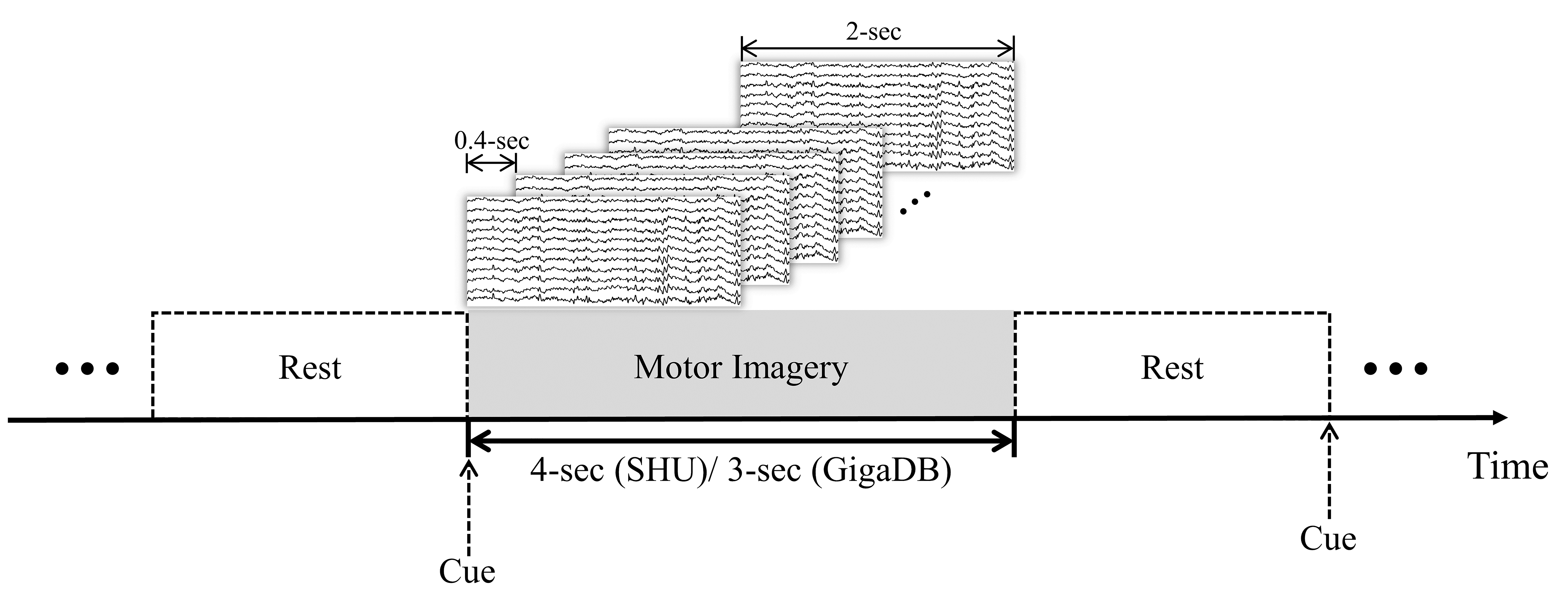 Fig. 1.
Sliding time window segmentation: 0.4-sec step, 2-sec width.
To capture brain network characteristics more effectively from EEG data, we selected features apt for depicting the state of brain networks: Pearson’s correlation coefficient, coherence, and phase-locking value. These metrics provide complementary measures of linear correlation, frequency correlation, and phase synchronization, respectively. Thus, the features derived from Pearson correlation coefficient, coherence, and phase locking value offer a holistic representation of the brain network’s connectivity state.
Pearson correlation coefficient (PCC) serves as a metric for measuring brain network features, evaluating the connectivity between brain regions by calculating the correlation between signals. The formula for PCC is as follows (Eqn. 1) [37]:
PCC is used to assess the linear relationship between two variables, reflecting their temporal interconnectedness. The calculation of PCC provides insights into the degree of direct linkage between different brain areas. The coefficient ranges from –1 to 1, where –1 indicates a perfect negative linear relationship, 0 signifies no linear correlation, and 1 indicates a perfect positive linear relationship.
Coherence (COH) serves as a measure to characterize time-frequency domain features, quantifying the similarity between components of two signals across different frequencies. The formula for COH is defined in Eqn. 2 [37]:
In this study, the COH method is applied for extracting temporal-frequency domain features. It evaluates the correlation or match between the frequency components of two distinct signals. This measure provides an indicator of the strength and consistency of the linear connection between two signals at various frequencies. COH represents the squared magnitude of the coherency function, calculated as the ratio of the power spectral density of the combined signals to the power spectral densities of the individual signals. The coherence value ranges from 0, indicating no correlation, to 1, denoting complete correlation at a specific frequency.
The phase locking value (PLV) method is employed for phase feature extraction. It measures the level of synchronization of signal phases, reflecting phase connectivity between neural regions. Notably, phase synchronization can occur even when signal amplitudes are uncorrelated. Despite the presence of noise and spontaneous phase shifts in practical applications, PLV accounts for the cyclic nature of phase. It produces values between 0, indicating a high variability in phase difference or low synchronization, and 1, signifying minimal variability or high synchronization. Therefore, for any given time t, the condition of phase-locking is described by Eqn. 3 [37]:
Where,
Accordingly, the PLV is a metric used to quantify the phase synchronization between two signals, indicating the consistency of their phase difference over time. The formula for PLV is given by Eqn. 5:
Where,
In summary, the combined use of PCC, COH, and PLV offers a comprehensive framework for analyzing the dynamic changes in EEG connectivity during motor imagery tasks. PCC focuses on linear connections, COH provides frequency-specific insights, and PLV reveals phase consistency. Together, these metrics allow for a detailed examination of the complex and dynamic activities within brain networks associated with motor imagery. This integrated approach enhances our understanding of the intricate dynamics present in brain networks during motor imagery tasks.
Considering the complexity of EEG signal characteristics in brain networks, we integrate the previously mentioned metrics, PCC, COH, and PLV, along with sliding time windows to construct a 3D brain network feature matrix, referred to as temporal-frequency-phase feature (TFPF). Fig. 2 illustrates the process of decoding TFPF features using the 3D-CNN-GAN model.
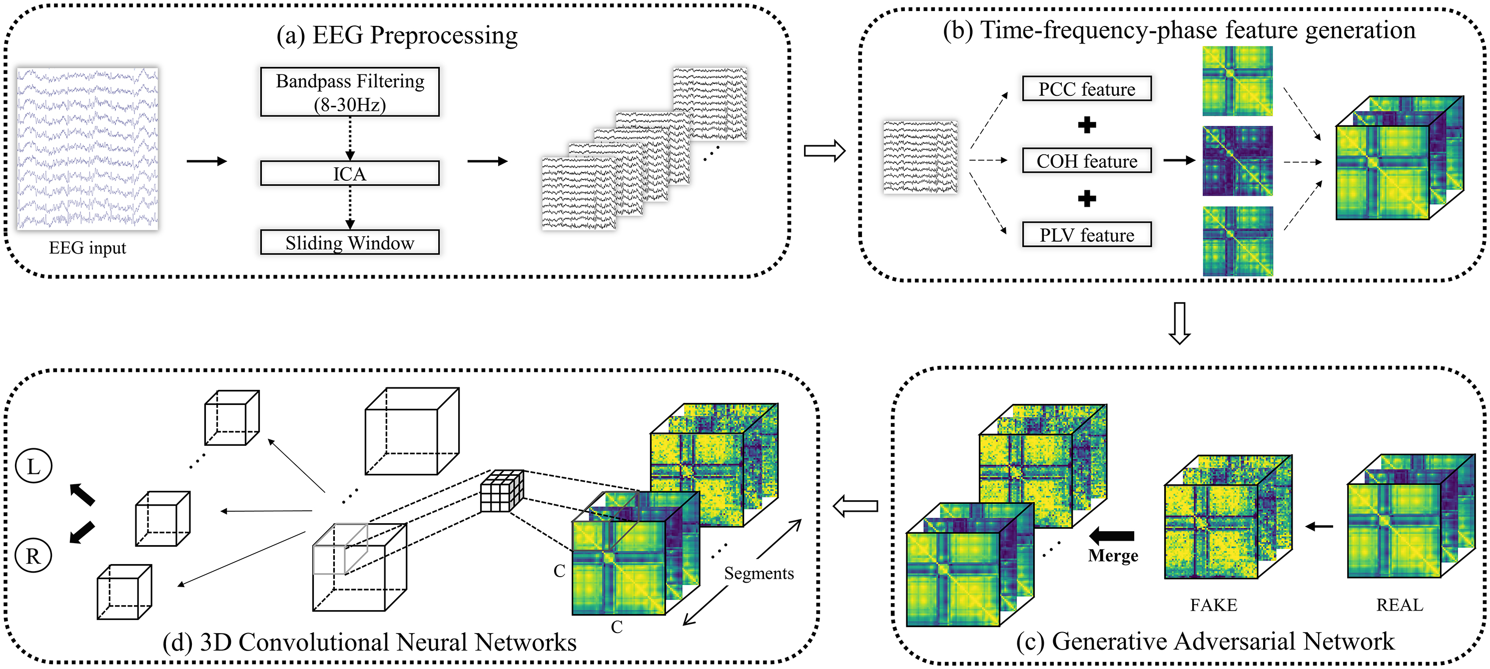 Fig. 2.
Schematic diagram of the 3D-CNN-GAN for decoding TFPF features. CNN, convolutional neural networks; GAN, generative adversarial networks; TFPF, temporal-frequency-phase feature; PLV, phase locking value; ICA, independent component analysis; PCC, pearson correlation coefficient; COH, coherence; EEG, electroencephalogram.
The sequential procedure of temporal-frequency-phase feature generation is as follows: After preprocessing, the EEG signals are analyzed to extract their temporal, spectral, and phase characteristics using PCC, COH, and PLV, respectively, forming the TFPF set. Concurrently, GANs are utilized to generate synthetic EEG signals. These GAN-generated signals undergo the same process of feature extraction (PCC, COH, and PLV) to form additional TFPF. Fig. 3 depicts the formation of TFPF and the resulting voxel segments.
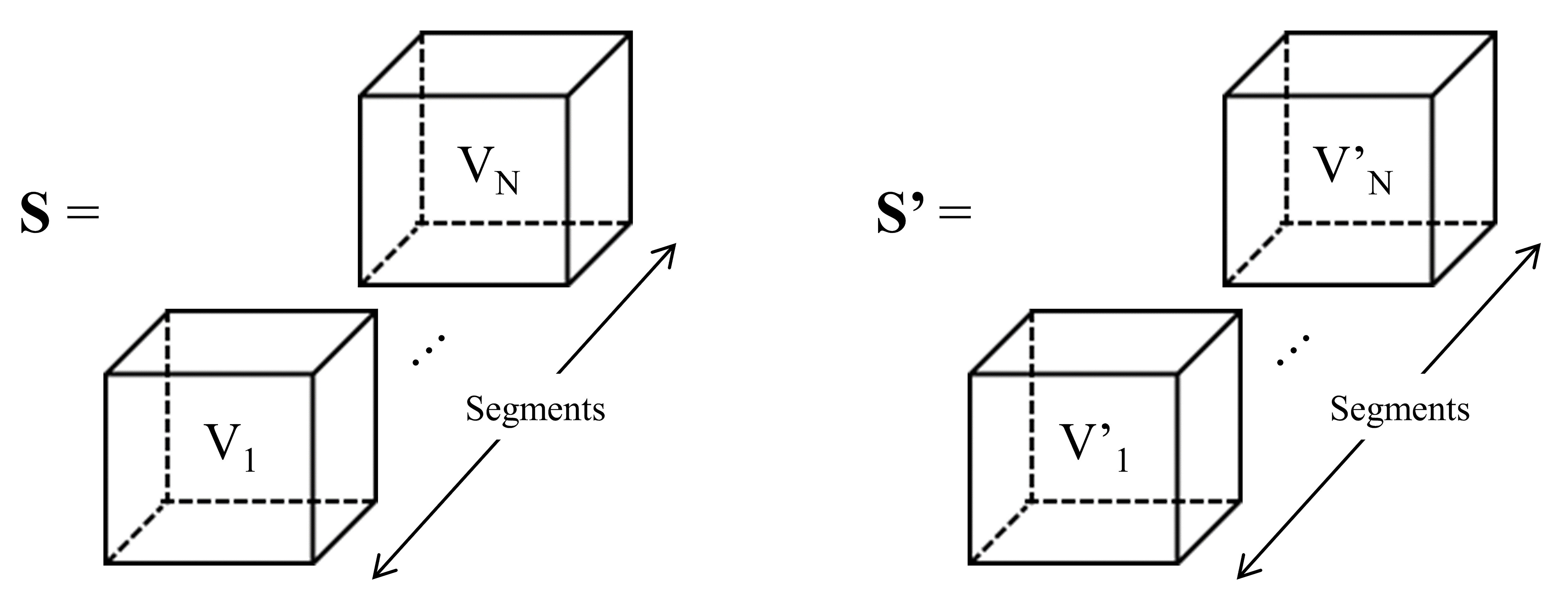 Fig. 3.
Process of forming TFPF. S represents the input set. Each voxel (V1, …, VN) is derived from EEG segments (Seg1, …, SegN). S’ represents the GAN-generated voxels. EEG, electroencephalogram.
Two types of TFPF voxels are produced: one voxel type (denoted as V) consists of EEG signals segmented by sliding time windows from the original input set (S), and the other voxel type (denoted as V’) is generated by the GAN (S’). Algorithm 1 outlines the detailed steps involved in the feature generation process:
This above Fig. 4 introduces a groundbreaking method for generating TFPF representations of EEG data and employing GANs to create synthetic TFPF representations. It involves calculating three types of features: PCC, COH, and PLV for each EEG segment. These features are stacked to form a unified feature vector for each segment. The REAL-TFPF representation is created by concatenating these feature vectors across all segments. Then, GANs are used to generate the FAKE-TFPF representation from the REAL-TFPF representation.
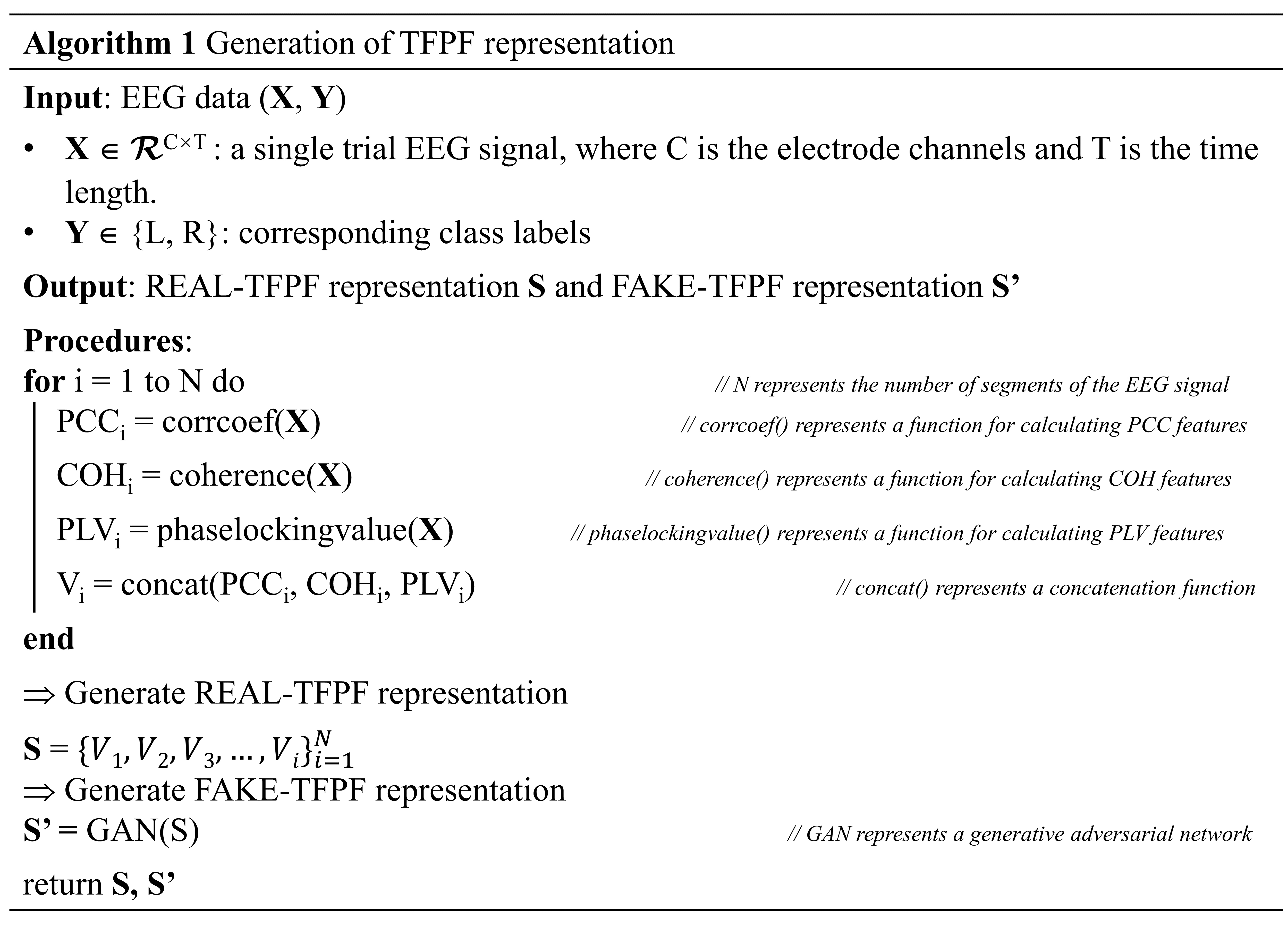 Fig. 4.
Generation of TFPF representation Algorithm. PCC, pearson correlation coefficient; COH, coherence; PLV, phase locking value.
The combined use of PCC, COH, and PLV metrics offers a powerful tool for exploring the brain’s connectivity and dynamics. This comprehensive approach not only facilitates the effective identification of EEG signal patterns but also aids in extracting vital insights into cognitive functions and underlying neural activities.
Employing a 3D-CNN for extracting multi-domain features represents a state-of-the-art method that amalgamates temporal, frequency, and phase data. The application of 3D-CNNs allows for the simultaneous capture of complex dynamics across these three domains, simplifying the feature extraction process and mitigating the potential reduction in accuracy associated with separate feature extraction techniques. Table 2 provides the implementation details of the 3D-CNN.
| Activation shape | Activation size | |
| Input: | (Nchannels, Nchannels, 3, 1) | Nchannels |
| C1 (k = [3, 3, 3], s = [1, 1, 1], p = ‘valid’) | (Nkernels, Nkernels, 1, 50) | Nkernels |
| C2 (k = [ Nkernels, Nkernels, 1], s = [1, 1, 1], p = ‘valid’) | (1, 1, 1, 100) | 100 |
C1: the first convolutional layer. C2: the second convolutional layer. k denotes kernel. s denotes stride. p denotes padding. Activation shape: (featurewidth, featurehigh, featurechannel, feature map). When employing SHU dataset, Nchannels = 32 Nkernels = 30; When employing GigaDB dataset, Nchannels = 60 Nkernels = 58.
Upon acquiring three-dimensional spectral features, the limitation of conventional 2D CNNs in fully preserving the intricate details of EEG signal information—spanning temporal, frequency, and phase domains—becomes evident. This shortfall overlooks the critical interdependence among the three dimensions. Consequently, this study adopts 3D CNNs to ensure the retention of complex, interrelated patterns essential for decoding cognitive states. The superior capability of 3D CNNs in feature extraction significantly enhances the model’s efficacy in detecting and categorizing brain activities related to motor imagery. This improvement leads to higher accuracy rates and more dependable real-time responses in BCI systems.
GANs have emerged as a significant technological advancement within the realm of BCIs, demonstrating substantial promise for a variety of applications, including data augmentation [38], signal denoising and decoding [39], neural rehabilitation, and brain-to-brain communication [4]. The key aspect of GANs is their objective function formula, as outlined below (Eqn. 6):
The GAN objective function is divided into two primary parts:
Discrimination of Real Data:
Ex∼pdata(x)[
Discrimination of Generated Data:
Ez∼pz(z)[
The architecture of GANs, characterized by its innovative generator-discriminator design, is adept at learning data distributions. This facilitates advancements in the creation of synthetic data and adversarial training methods. The intricate architecture of GANs, as applied to the GigaDB and SHU datasets, is detailed in Tables 3a,3b,4a,4b.
| Layer | Output Shape | Param |
| Conv2D | (None, 30, 30, 128) | 3584 |
| Leaky Relu | (None, 30, 30, 128) | 0 |
| Conv2D | (None, 15, 15, 128) | 147,584 |
| Leaky Relu | (None, 15, 15, 128) | 0 |
| Flatten | (None, 28800) | 0 |
| Dropout | (None, 28800) | 0 |
| Dense | (None, 1) | 28,801 |
| Total params: 179,969 | ||
| Trainable params: 179,969 | ||
| Non-trainable params: 0 | ||
| Layer | Output Shape | Param |
| Dense | (None, 28,800) | 2,908,800 |
| LeakyRelu | (None, 28,800) | 0 |
| Reshape | (None, 15, 15, 128) | 0 |
| Conv2D Transpose | (None, 30, 30, 128) | 262,272 |
| LeakyRelu | (None, 30, 30, 128) | 0 |
| Conv2D Transpose | (None, 60, 60, 128) | 262,272 |
| LeakyRelu | (None, 60, 60, 128) | 0 |
| Conv2D | (None, 60, 60, 3) | 24,579 |
| Total params: 3,457,923 | ||
| Trainable params: 3,457,923 | ||
| Non-trainable params: 0 | ||
| Layer | Output Shape | Param |
| Conv2D | (None, 16, 16, 128) | 3584 |
| LeakyRelu | (None, 16, 16, 128) | 0 |
| Conv2D | (None, 8, 8, 128) | 147,584 |
| LeakyRelu | (None, 8, 8, 128) | 0 |
| Flatten | (None, 8192) | 0 |
| Dropout | (None, 8192) | 0 |
| Dense | (None, 1) | 8193 |
| Total params: 159,361 | ||
| Trainable params: 159,361 | ||
| Non-trainable params: 0 | ||
| Layer | Output Shape | Param |
| Dense | (None, 8192) | 827,392 |
| LeakyRelu | (None, 8192) | 0 |
| Reshape | (None, 8, 8, 128) | 0 |
| Conv2D Transpose | (None, 16, 16, 128) | 262,272 |
| Leaky Relu | (None, 16, 16, 128) | 0 |
| Conv2D Transpose | (None, 32, 32, 128) | 262,272 |
| Leaky Relu | (None, 32, 32, 128) | 0 |
| Conv2D | (None, 32, 32, 3) | 24,579 |
| Total params: 1,376,515 | ||
| Trainable params: 1,376,515 | ||
| Non-Trainable params: 0 | ||
The integration of Generative Adversarial Networks with 3D-CNN-GAN creates a formidable strategy for dataset augmentation through the generation of an enriched set of TFPF. The GAN, recognized for its proficiency in data augmentation, is adept at creating an enrich set of TFPF that accurately replicate the intricate properties of original EEG signals. This capability significantly enhances the volume and quality of training data, which in turn improves the motor imagery decoder’s ability to generalize and perform classifications. By merging GAN with 3D-CNN, the combined framework exploits the comprehensive analytical power of three-dimensional convolution, capturing a more detailed representation of EEG signal dynamics across various domains. The strategic emphasis on the 3D-CNN-GAN architecture not only extends the dataset with quality features but also strengthens the classification mechanism. This approach offers a sophisticated method for decoding the complex patterns present in EEG data.
Within the realm of EEG signal
classification, it has been observed that shallow network architectures often
outperform deeper networks, a trend that contrasts with observations in other
tasks. In line with this finding, we have meticulously designed a neural network
with just two convolutional layers, as shown in Fig. 2d. The initial
convolutional layer features a kernel voxel size of 3
To validate our model’s stability and accuracy, for both GigaDB and SHU datasets in a within-session scenario, we divided the independent data segments into two equal parts; 50% were enhanced using a GAN network [40], resulting in an augmented set of twofold independent data segments for training. The remaining 50% independent data segments were used for testing. Hence, for the 3D-CNN-GAN, under the within-session scenario, the training data from both GigaDB and SHU datasets accounts for 2/3 of the total dataset, while the testing data accounts for 1/3 of the total dataset. For the cross-session scenario, each of the five sessions per subject is split into two equal parts due to the sliding time window strategy. We enhanced the independent data segments from the four sessions not involved in testing using GAN. Consequently, for the 3D-CNN-GAN in a cross-session scenario within the SHU dataset, each experiment’s training data accounts for 8/9 of the total dataset, with test independent data segments comprising 1/9. Therefore, this approach ensures our model’s robustness and dependability, as well as the relevance of our test data, thereby affirming the model’s credibility.
Our comprehensive brain network analysis meticulously examined the complex interconnectivity and nuanced information flow within the brain. This examination helped uncover interactions among various brain regions, elucidating the pathways of information transfer and the collaborative operations of neural functions. This contributes to our understanding of the foundational processes that govern cerebral functionality and cognitive dynamics. Fig. 5 illustrates the brain network analysis process, beginning with EEG signal processing to extract features, followed by calculating the connectivity between different brain regions, and concluding with the analysis of the differences between real and fake brain connectivity.
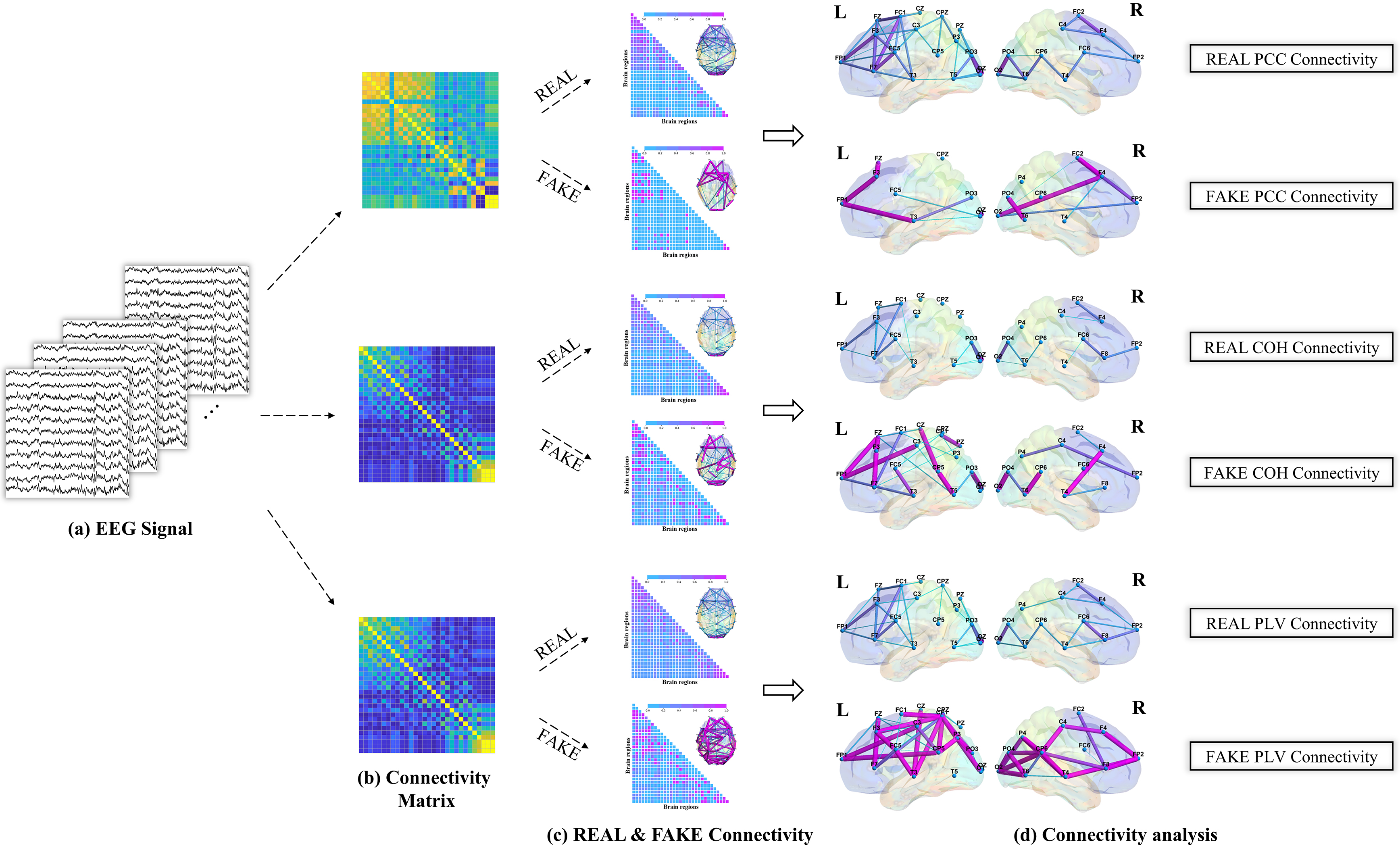 Fig. 5.
Schematic diagram of brain network analysis. (a) Clean EEG signal was obtained. (b) Multi-domain feature representation for the connectivity matrix. (c) REAL & FAKE Connectivity Assessment. (d) REAL & FAKE connectivity analysis using significant connections based on PCC, COH, and PLV. PCC, pearson correlation coefficient; COH, coherence; PLV, phase locking value; L, left hand; R, right hand.
In this section, we evaluate the 3D-CNN and the proposed 3D-CNN-GAN models by their classification accuracy, detailed by both session and subject within the SHU dataset and GigaDB dataset. We then performed a brain network analysis to investigate the topology of the brain network and the experimental results corresponding to this analysis. Additionally, we explored the impact of GAN on the characteristics of brain network connectivity, specifically examining the interpretable similarities between REAL and FAKE connections.
To assess the efficacy of the proposed 3D-CNN and 3D-CNN-GAN models in handling EEG session variability, we conducted classification experiments across multiple sessions using the SHU and GigaDB datasets, as shown in Figs. 6,7.
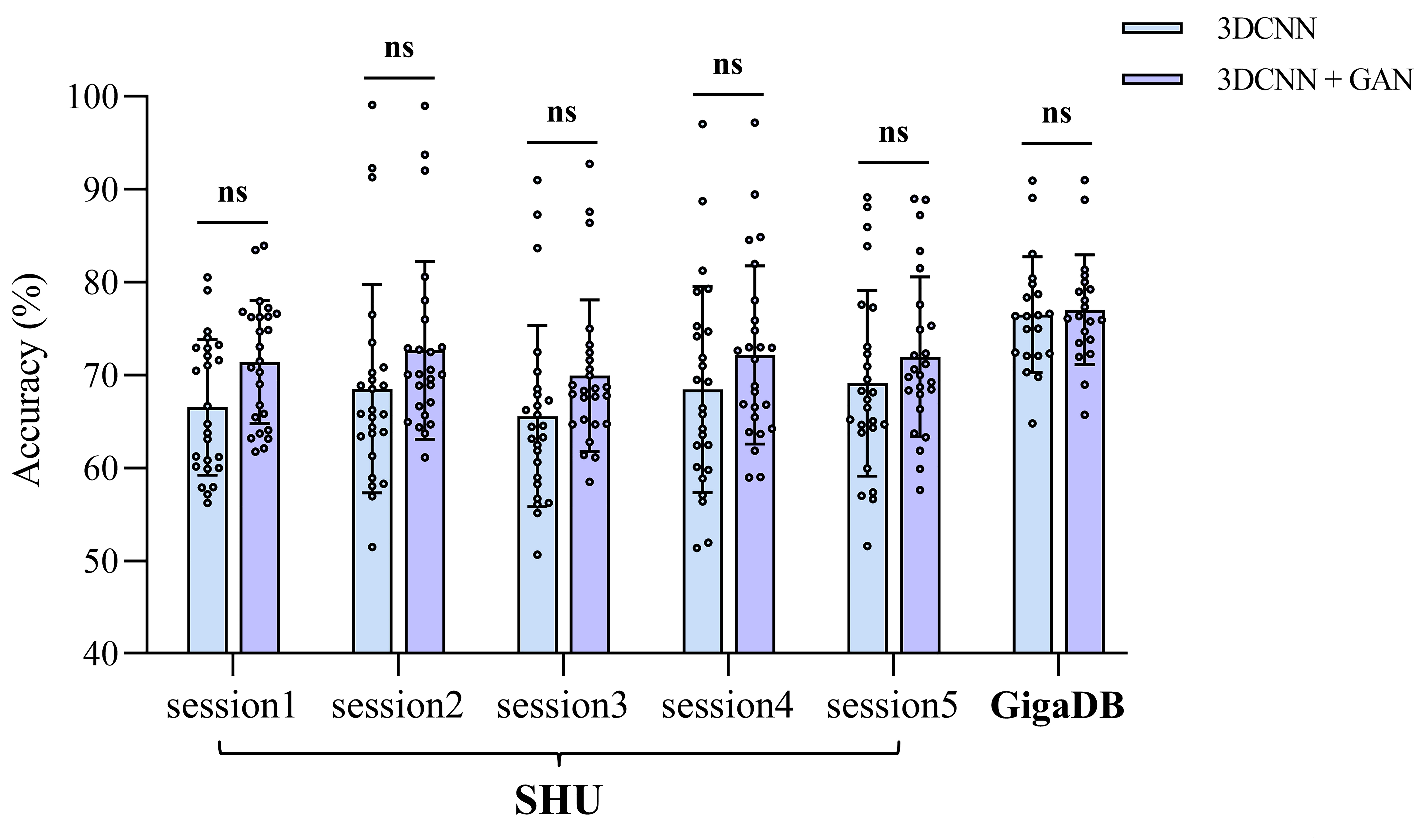 Fig. 6.
The comparison of average within-session classification accuracies between 3D-CNN and 3D-CNN-GAN across the two datasets, detailing the performance for each session. NS indicates no significant difference.
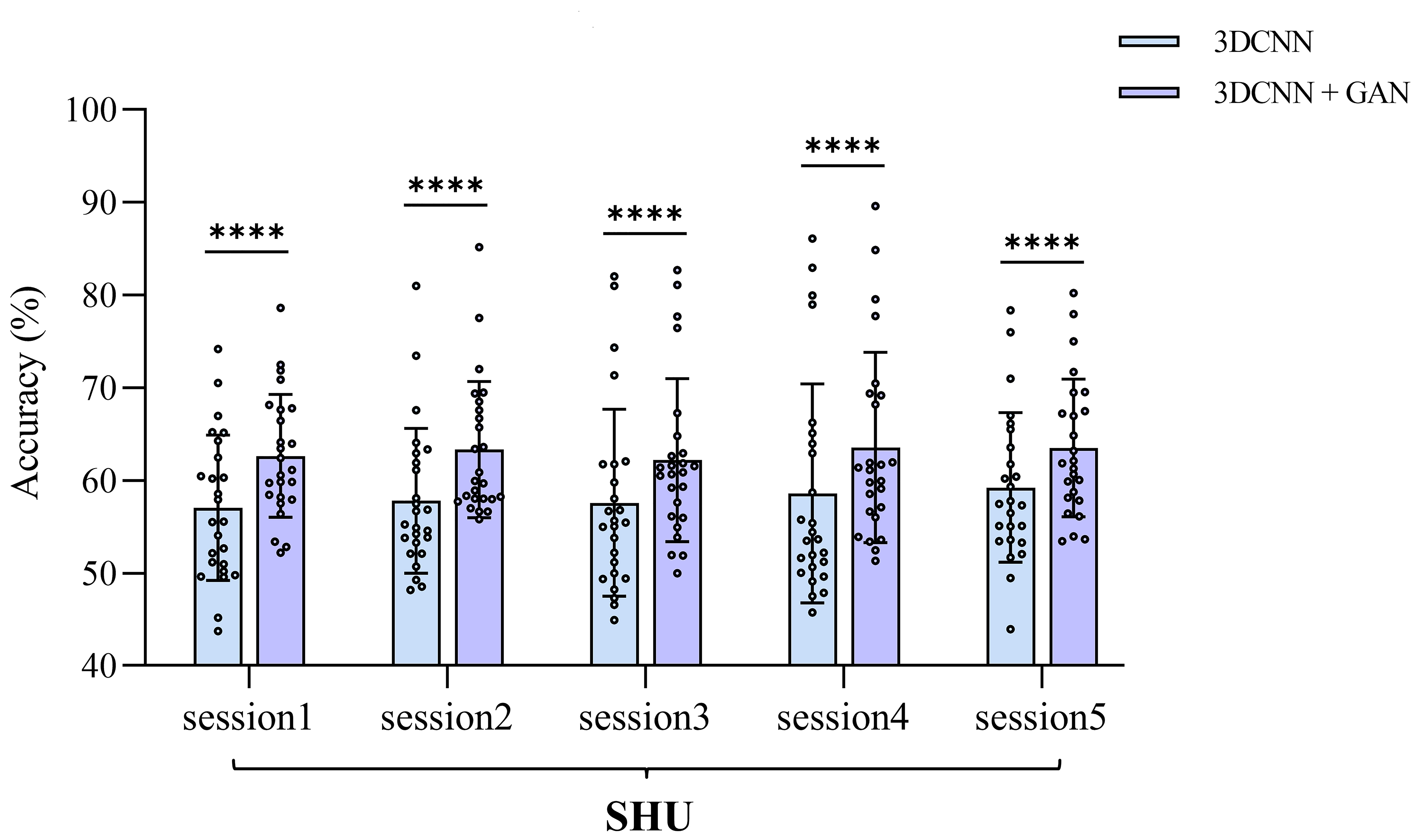 Fig. 7.
The comparison of average cross-session classification
accuracies between 3D-CNN and 3D-CNN-GAN within the SHU dataset, detailed for
each session. **** indicates p
In the SHU dataset, the 3D-CNN-GAN model shows a notable improvement in classification accuracy, with within-session improvements of up to 3.99% and cross-session improvements of up to 4.98%. However, in the GigaDB dataset, the improvement with the 3D-CNN-GAN model is not as pronounced, with the 3D-CNN and 3D-CNN-GAN models achieving accuracies of 76.59% and 77.03%, respectively. The marked improvement observed in the SHU dataset can be attributed to the GAN’s ability to enhance the learning of brain network connectivity features and effectively eliminate irrelevant connections, likely due to potential external interferences encountered during EEG data collection in the SHU dataset.
To assess the 3D-CNN and 3D-CNN-GAN models’ ability to manage EEG variability across individuals, classification experiments were conducted for each subject within the SHU and GigaDB datasets. Fig. 8 shows a detailed analysis of classification accuracies for individual subjects across these two datasets, employing both 3D-CNN and 3D-CNN-GAN models. In the GigaDB dataset, the average within-session classification accuracy using 3D-CNN stands at 76.49%, with a slight increase to 77.03% observed when employing the 3D-CNN-GAN model. Notably, within this average, subjects S3 and S14 reached exceptional average accuracies of 88.87% and 91%, respectively. Conversely, in the SHU dataset, the 3D-CNN model’s within-session average accuracy of 67.42% improved to 71.63% with the 3D-CNN-GAN, and for cross-session, the average accuracy rose from 58.06% with 3D-CNN to 63.04% with 3D-CNN-GAN. A closer look reveals that, despite the overall average accuracy of 71.63% for within-session and 63.04% for cross-session with the 3D-CNN-GAN model, significant exceptions were observed. For instance, within the SHU dataset, subject S6 achieved accuracies of 88.27% within-session and 80.55% cross-session, while subject S16 reached accuracies of 84.29% within-session and 78.68% cross-session. These significant improvements in the SHU dataset highlight the GAN algorithm’s effectiveness, especially in enhancing classification accuracy per subject. The uniform improvement across all subjects in the SHU dataset with the 3D-CNN-GAN model evidences the algorithm’s capability to bolster the discriminative features of EEG signals for motor imagery classification.
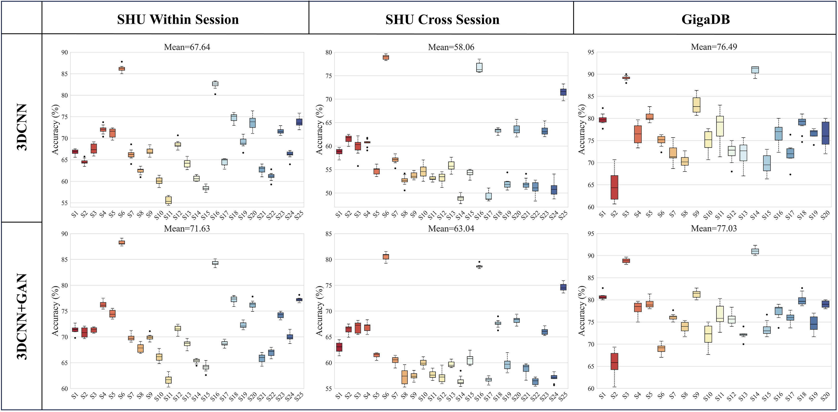 Fig. 8.
Comparison of within-session and cross-session classification accuracies for 3D-CNN and 3D-CNN+GAN across two datasets, detailed for each subject.
Upon examining the subject-specific experimental results shown in Fig. 8, it is evident that SHU-S6 achieved the highest accuracy, with significant improvements attributed to GAN. Consequently, we delved deeper into the analysis of the best performer’s brain network features, revealing the reasons behind its superior performance from the perspective of brain functional connectivity. This approach facilitates an understanding and observation of the neural mechanisms underlying effective classification performance in motor imagery tasks. Analyzing connectivity metrics provides valuable insights into the collaboration and cooperation among brain regions involved in motor imagery tasks.
In this research, our research team explored brain functional connectivity by extensively analyzing the brain network of SHU-S6 from the SHU dataset. Fig. 9 presents the lateral view of brain network topology, combining PCC, COH, and PLV with GAN, to depict the connectivity across different brain regions through the color and line thickness of the marked lines.
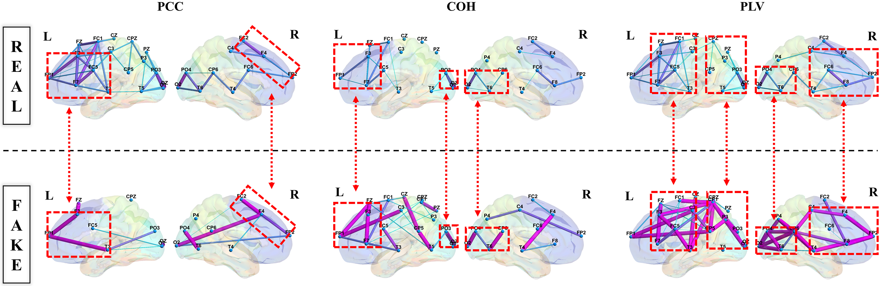 Fig. 9.
Lateral view of brain network topology.
Our investigation revealed that the connections between key brain regions, such as the frontal, parietal, and occipital lobes, intensified during motor imagery tasks. Notably, Fig. 9 contrasts the “REAL Connectivity” and “FAKE Connectivity” within the brain network, revealing that the latter often exhibited a greater number of structures and stronger connections. Specifically, enhanced connectivity was particularly noted between the prefrontal motor area, the parietal lobe’s somatosensory associated area, and the occipital lobe’s visual associated area and visual cortex.
Upon further observation, it is exciting to note the formation of “triangular structures” and “circular structures”. Specifically, there was an observed enhancement in connectivity between the prefrontal motor area, the somatosensory associated area of the parietal lobe, and the visual associated area along with the visual cortex of the occipital lobe. Further examination revealed the intriguing formation of “triangular structures” and “circular structures” within the highlighted red border regions of the frontal, parietal, and occipital lobes. These structures are pivotal characteristics of complex networks, and an increased number of such structural features within brain connectivity signifies enhanced stability in “communication” across different brain regions. This revelation holds significant implications for a deeper understanding of EEG features and their application in brain network analysis, offering new strategies to enhance classification accuracy.
Furthermore, compared with the brain network topology of REAL and FAKE Connectivity, add the top view brain network topology and the corresponding adjacency matrix. In Fig. 10, we analyzed the network structural features using data from SHU dataset subject S6. The color and thickness of the marked lines represent the connectivity strength of different brain regions from top view brain network topology, combined with the corresponding adjacency matrix, connectivity structures, and strength of “FAKE Connectivity”, which are stronger compared to “REAL Connectivity”. Thus, from the confirmed experimental insights, we found that combining PCC, COH, and PLV with GAN not only augments the volume of data available for analysis but also potentially enriches the feature content with synthesized EEG signals that exhibit similar spectral and temporal characteristics as the real data. Experimental results confirmed that this approach not only markedly improved classification accuracy within the SHU dataset but also enhanced the model’s interpretability.
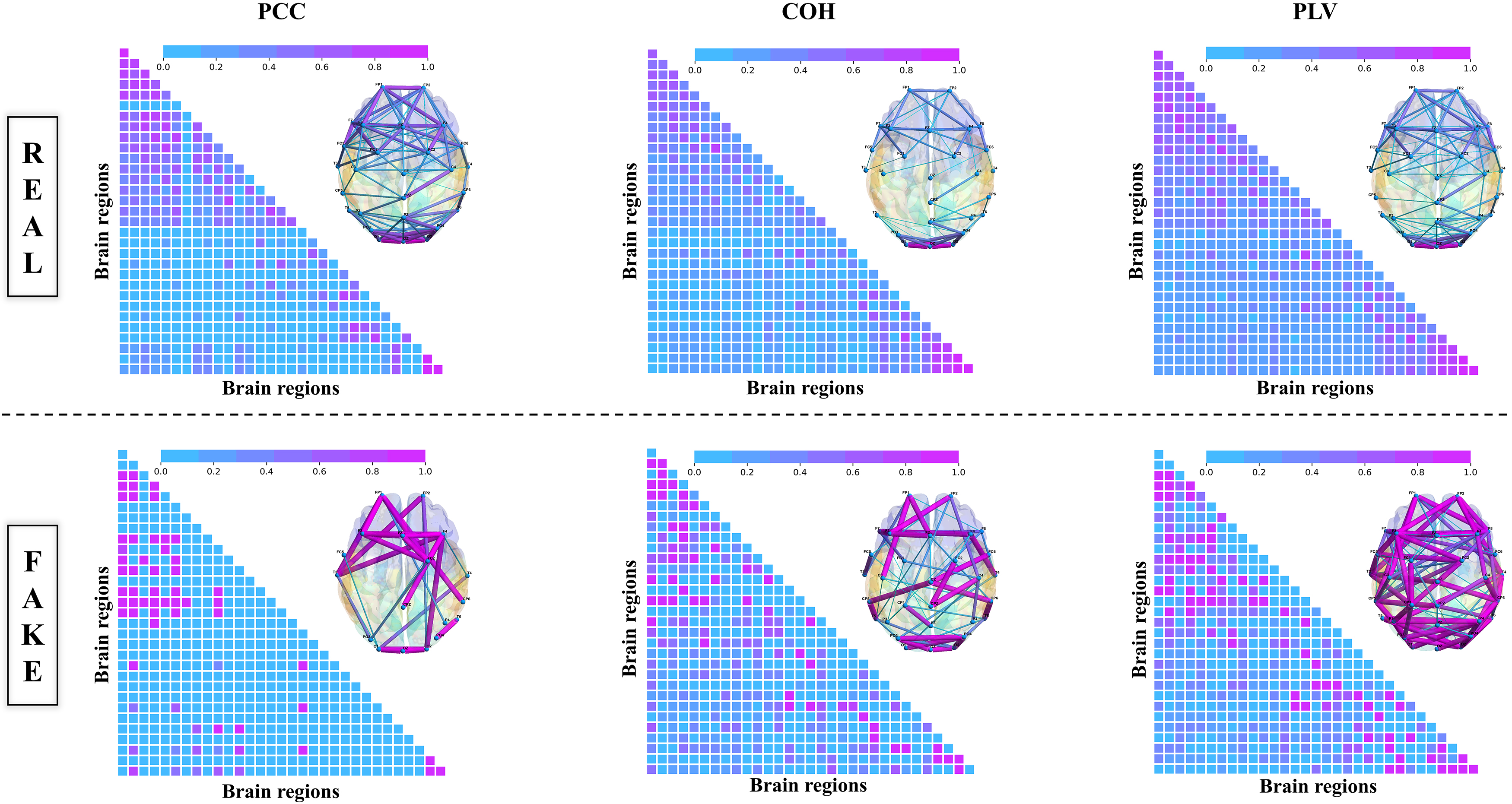 Fig. 10.
Top view of brain network topology.
In this study, we introduced a novel framework employing a 3D-convolutional neural network combined with a 3D-CNN-GAN for the enhancement and classification of motor imagery tasks. This framework excels at integrating brain network features with deep learning and GANs to decode motor imagery EEG signals.
To clarify these findings, we conducted classification experiments at both individual and session levels using the SHU and GigaDB datasets. Specifically, at the individual level, the experiments assessed the proposed model’s generalization capability across different individuals. The preprocessing of EEG signals for each time window involved the analysis to extract PCC, COH, and PLV features, which were then integrated to form a 3D feature representation. The GAN is designed to generate synthetic EEG features indistinguishable from real data, thus enlarging the training dataset and improving the model’s generalization ability. This approach effectively captures the temporal, frequency, and phase-related features of EEG signals, simplifying the inherent complexity of EEG data analysis. Furthermore, a 3D-CNN model with two convolutional layers was utilized to classify two-class motor imagery tasks based on the TFPF. The results, as shown in Tables 5,6 (Ref. [8, 11, 12, 26, 41, 42, 43, 44, 45, 46]), demonstrate that the proposed 3D-CNN-GAN method outperforms existing research methodologies. These results highlight the method’s efficacy in motor imagery classification and its ability to decode within-session variability patterns (within-session-level) and cross-session variability patterns (cross-session-level).
| Method | Subjects | Level | Avg.ACC | Dataset |
| FBCNet [41] | 25 | WS | 68.85% | SHU |
| CSP [26] | 25 | WS | 57.33% | |
| WTS-SVM [42] | 25 | WS | 65.51% | |
| FBCSP [8] | 25 | WS | 64.33% | |
| EEGNet [11] | 25 | WS | 65.03% | |
| DeepConvNet [12] | 25 | WS | 64.82% | |
| Bi-LSTM [42] | 25 | WS | 61.83% | |
| Proposed method | ||||
| 3D-CNN [43] | 25 | WS | 67.42% | |
| 3D-CNN-GAN | 25 | WS | 71.63% | |
| OPTICAL [44] | 52 | WS | 68.19% | GigaDB |
| D&W CNN [45] | 26 | WS | 76.21% | |
| Proposed method | ||||
| 3D-CNN [43] | 20 | WS | 76.49% | |
| 3D-CNN-GAN | 20 | WS | 77.03% |
WS, within-session testing; Avg.ACC, Average Accuracy; FBCNet, Filter Bank Convolutional Network; WTS-SVM, Wavelet Time Scattering-based Support Vector Machine; CSP, common spatial pattern; SVM, support vector machine; FBCSP, filter bank common spatial pattern; EEG, electroencephalogram; LSTMs, long short-term memory networks; CNN, convolutional neural networks; GAN, generative adversarial network; OPTICAL, Optimized and LSTM based predictor; D&W; Deep and Wide.
| Method | Subjects | Level | Avg.ACC | Dataset |
| MEIS [46] | 25 | CS | 58.83% | SHU |
| FBCNet [41] | 25 | CS | 50.97% | |
| CSP [46] | 25 | CS | 51.16% | |
| WTS-SVM [42] | 25 | CS | 59.38% | |
| EEGNet [11] | 25 | CS | 53.65% | |
| DeepConvNet [12] | 25 | CS | 52.92% | |
| Bi-LSTM [42] | 25 | CS | 53.91% | |
| CSA [26] | 25 | CS | 57.56% | |
| Proposed method | ||||
| 3D-CNN [43] | 25 | CS | 58.06% | |
| 3D-CNN-GAN | 25 | CS | 63.04% |
CS, cross-session testing; MEIS, Manifold Embedded Instance Selection Algorithm; CSA, cross session adaptation.
It is noteworthy that, as Table 5 shows, under within-session conditions, the 3D-CNN-GAN algorithm outperforms the existing state-of-the-art decoding algorithms in the literature for both SHU and GigaDB datasets. Furthermore, Table 6 illustrates that under cross-session conditions, the decoding accuracy improvement by the 3D-CNN-GAN algorithm becomes more pronounced, highlighting the benefits of incorporating GANs in addressing session-variability issues. However, the GigaDB dataset, comprising only a single session per subject, did not allow for cross-session testing. Conversely, in cross-session classification, discussing transfer learning methodology is essential. Ma et al. [26]. employed transfer learning, termed cross session adaptation (CSA), for testing. In the SHU dataset, with time intervals between each of the five sessions per subject ranging from 2 to 3 days, significant differences in feature distribution across sessions were observed. For the CSA algorithm in Ma et al. [26], if the adaptation data partition includes test set trials, the feature distribution within the same session can be effectively recognized by the transfer learning base model, resulting in better adaptation outcomes. In contrast, our training strategy treats the five sessions as separate entities, excluding the test session from the training process. This approach did not show improvement in the CSA method’s efficacy in our tests.
Moreover, the 3D-CNN-GAN stands out with several advantages over other state-of-the-art methods. Firstly, its 3D aspect integrates three crucial brain network parameters: PCC, COH, and PLV, providing a comprehensive view of dynamic EEG connectivity changes during motor imagery. PCC delineates linear relationships, COH reveals frequency-specific synchronization, and PLV highlights phase consistency across EEG signals, together forming a robust feature set for neural network analysis. Secondly, the deep learning CNN model, a core component of the framework, enhances interpretability, often a challenge in neural decoding tasks. It bridges the gap between raw EEG data and the abstract representations learned by deep neural networks, thus improving the model’s output interpretability, as illustrated in Figs. 9,10. Lastly, the inclusion of a GAN overcomes the large dataset dependency typical of deep learning models. The GAN generates synthetic EEG features, enhancing the training dataset and generalization capabilities, vital in EEG analysis where large, diverse datasets are scarce. The synergy between generated and original brain network features offers a validation mechanism, ensuring model robustness by assessing the synthetic data’s reliability and authenticity.
Acknowledging the limitations of our study is crucial for the interpretation of our findings. The preprocessing procedures, such as filtering, significantly contribute to the proposed method’s performance; thus, further exploration of various preprocessing methods is vital to fully understanding their impact on classification accuracy. Additionally, the study utilized relatively small datasets, necessitating an assessment of the method’s scalability and efficiency with larger datasets to determine its practical applicability in real-world scenarios.
In conclusion, our study explored the 3D-CNN-GAN model’s effectiveness in classifying motor imagery tasks using brain network features, PCC, COH, and PLV, extracted from the GigaDB and SHU datasets. The GAN network substantially enhanced classification accuracies both within and across sessions on the SHU dataset, noted for its laboratory-induced noise, and achieved a modest improvement in within-session classification on the public GigaDB dataset. These findings demonstrate the GAN’s capability to learn motor imagery features effectively, particularly in noisy settings, thus confirming the robustness of the 3D-CNN-GAN framework and its potential applicability in real-world BCI scenarios.
Future work should address several areas. Primarily, assessing the 3D-CNN-GAN framework’s efficacy and real-time applicability in real-world environments is essential, with a particular focus on GAN implementation. The integration of brain networks with deep learning and GAN techniques is expected to gain considerable interest in the BCI research community. Further research directions include applying the 3D-CNN-GAN architecture to diverse EEG-based BCI applications, such as emotion recognition and cybersecurity. The proposed TFPF feature sets, coupled with CNN’s deep learning capabilities and GAN’s data augmentation, show potential for capturing essential multi-domain dynamics for specific tasks, making this integrated approach versatile for various BCI applications.
The data sets analyzed during the current study are available in the GigaDB repository and SHU repository. GigaDB dataset is publicly available at http://gigadb.org/dataset/100295. SHU dataset is publicly available at https://figshare.com/articles/software/shu_dataset/19228725.
CF designed the experiment and carried out the overall design and writing of the paper. BY provided paper ideas and 3D-CNN-GAN framework for writing. XL provided brain network analysis and validation. SG provided generative adversarial network code inspection. PZ refined the ideas and provided the manuscript revision. All authors contributed to editorial changes in the manuscript. All authors read and approved the final manuscript. All authors have participated sufficiently in the work and agreed to be accountable for all aspects of the work.
Not applicable.
Thank you for the administrative support of the graduate school at Shanghai University and the technical support provided by MathWorks and Jetbrains. Additionally, I would like to thank my lab colleagues’ valuable technical advices and my family’s unwavering support.
This research was funded by National Key Research and Development Program of China (2022YFC3602500, 2022YFC3602504), National Natural Science Foundation of China (No. 62376149).
The authors declare no conflict of interest.
References
Publisher’s Note: IMR Press stays neutral with regard to jurisdictional claims in published maps and institutional affiliations.