


1 School of Mathematical Sciences, Soochow University, 215006 Suzhou, Jiangsu, China
2 Zu Chongzhi Center, Duke Kunshan University, 215316 Kunshan, Jiangsu, China
3 Department of Mathematics and Statistics, York University, Toronto, ON M3J 1P3, Canada
4 Department of Applied Mathematics, Illinois Institute of Technology, Chicago, IL 60616, USA
5 Math and Statistics Department, Utah State University, Old Main Hill, Logan, UT 84322, USA
Abstract
Ion and water transport in the central nervous system (CNS) is governed by tightly coupled mechanisms involving electrodiffusion, osmotic pressure, and fluid convection. Disruptions to these processes are implicated in pathological conditions. Understanding the coordinated roles of glial cells and perivascular spaces in regulating ionic and fluid homeostasis is essential for interpreting neural function and dysfunction.
We developed a multicompartment model of the optic nerve incorporating axons, glial cells, extracellular space (ECS), and three perivascular compartments (arterial, venous, and capillary-associated). The model integrates electrodiffusion of ions, osmotic water transport, and convection, while enforcing electroneutrality and compartmental volume conservation. Numerical simulations were performed using a finite volume method under axisymmetric geometry, and parameter sensitivity was explored through variations in glial membrane conductance, connexin permeability, and aquaporin-4 (AQP4) expression.
The simulations reveal that potassium released from axons during stimulation is cleared via glial uptake and redistributed through electric drift within glial syncytia. The perivascular pathway provides a secondary route for potassium and water clearance. Decreased glial conductance leads to abnormal firing in unstimulated axons, mimicking epileptiform activity, while reduced connexin coupling increases dependence on perivascular drainage. Changes in AQP4 expression had limited effect on ionic homeostasis in the current model.
This model provides a biophysically consistent framework to study ionic-fluid coupling in CNS microcirculation. It demonstrates how glial and perivascular compartments cooperate to maintain extracellular potassium balance. The findings offer insight into the mechanisms underlying pathological K+ accumulation and suggest potential therapeutic targets involving glial modulation and perivascular enhancement. The framework is extensible to other brain regions and conditions involving impaired clearance or excitability.
Keywords
- potassium
- glial cells
- ion transport
- water-electrolyte balance
- mircociruclation modeling
Potassium clearance plays a pivotal role in maintaining the stability and functionality of the central nervous system (CNS) [1]. In the resting state, nerve cells maintain a polarized membrane potential, with the interior of the cell negatively charged relative to the outside. This polarization arises from the unequal distribution of key ions—primarily Na+, K+, and Cl–—across the cell membrane, as well as the selective permeability of ion channels and the action of ion pumps. During an action potential, depolarization occurs when voltage-gated Na+ channels open, allowing a rapid influx of Na+ ions into the cell. This inward positive current reduces the membrane potential difference, bringing it toward or above zero. Subsequently, voltage-ated K+ channels open. Repolarization is primarily driven by the efflux of K+ ions through potassium channels, which restores the negative internal potential. Cl– ions, depending on their electrochemical gradient, may also contribute to membrane hyperpolarization by moving inward and counteracting depolarization. Proper potassium regulation is critical for stabilizing neuronal membrane potentials, enabling action potential generation and synaptic transmission. During heightened neuronal activity, potassium ions (K+) are released into the extracellular space (ECS). Without timely clearance, this excess potassium can accumulate, causing pathological depolarization, neuronal hyperexcitability, and potentially trigger seizures.
Glial cells, particularly astrocytes, are essential for potassium clearance in
the CNS, including the optic nerve [2]. Through connexin-based gap junctions,
astrocytes form a syncytium that facilitates the redistribution and buffering of
potassium ions within the ECS [3]. This process is closely coupled to fluid flow
within the glymphatic system, where aquaporin-4 (AQP4) channels in astrocytic
endfeet regulate water movement [4, 5]. The glymphatic system enables
cerebrospinal fluid (CSF) influx through perivascular spaces (PVS), facilitating
the clearance of metabolic waste products such as amyloid-
The optic nerve, as part of the CNS, shares structural similarities with the brain, including its narrow ECS and surrounding glial cells [11]. It consists of four regions: the intraocular nerve head, intraorbital, intracanalicular, and intracranial regions [12]. This study focuses on the intraorbital region, which constitutes the majority of the optic nerve. CSF enters the optic nerve through perivascular spaces surrounding blood vessels, interacting with glial cells lining these spaces [13]. This dynamic flow is essential for potassium clearance and waste removal, processes that, when impaired, are associated with conditions such as glaucoma [14].
Mathematical models have been developed to study potassium clearance and spatial buffering, focusing primarily on fluid dynamics and ionic transport. Early models examined fluid flow within the perivascular spaces, often driven by arterial pulsations [15, 16]. More recently, machine learning approaches have been employed to explore mechanisms in the glymphatic system [17, 18], as comprehensively reviewed in [19]. However, these models exhibit notable limitations. They often neglect the complex interaction between different compartments—such as the ECS, glial cells, and perivascular spaces—and fail to incorporate critical processes such as electric drift and osmotic effects. Electric drift redistributes potassium ions along electrochemical gradients within the glial compartment [20], while osmotic pressure drives water movement in response to ion concentration changes, maintaining ECS volume and astrocyte function [21]. Collectively, these mechanisms ensure efficient potassium clearance and prevent pathological K+ accumulation, which can otherwise lead to hyperexcitability, excitotoxicity, and cerebral edema formation.
To address these gaps, we developed a multidomain mathematical model that integrates six compartments: axons, glial cells, the extracellular space, and three perivascular spaces (PVS A, V, and C). Building upon the tridomain framework introduced by Zhu et al. [22], our model integrates the interplay between ionic electrodiffusion, osmosis, and fluid circulation. By incorporating the dynamics of glial function and glymphatic pathways, this model provides a comprehensive framework for elucidating potassium clearance mechanisms in the optic nerve.
Additionally, our model considers the interaction between the optic nerve and surrounding cerebrospinal fluid, which flows through the perivascular spaces and subarachnoid space (SAS) as part of the glymphatic pathway [23]. By differentiating between extracellular and perivascular spaces and accounting for direct communication between CSF and PVS A and V, we aim to enhance our understanding of glymphatic function in response to neural activity and potassium clearance.
Despite its advancements, the current model has limitations. It assumes spatial homogeneity in the glial compartment and perivascular spaces, neglecting regional variations in permeability, conductivity, and ionic gradients. Furthermore, the simplified representation of potassium channels does not capture the diversity of channel subtypes and their biophysical properties. Additionally, biochemical processes such as enzyme activity and metabolite interactions, which may influence waste clearance, remain excluded. Future refinements addressing these limitations will enhance the model’s predictive capacity and applicability to pathological conditions such as neurodegeneration.
The remainder of this article is organized as follows: Section 2 describes the mathematical model for potassium and fluid microcirculation in the optic nerve. Section 3 presents simulation results, focusing on the effects of glial cells and perivascular spaces on potassium clearance. Finally, Section 4 provides concluding remarks and discusses directions for future work.
Fig. 1 shows the structure we are modeling. This is a subset of all the
structures of interest in the optic nerve, but it is a good place to start.
Computational domain
where the domain
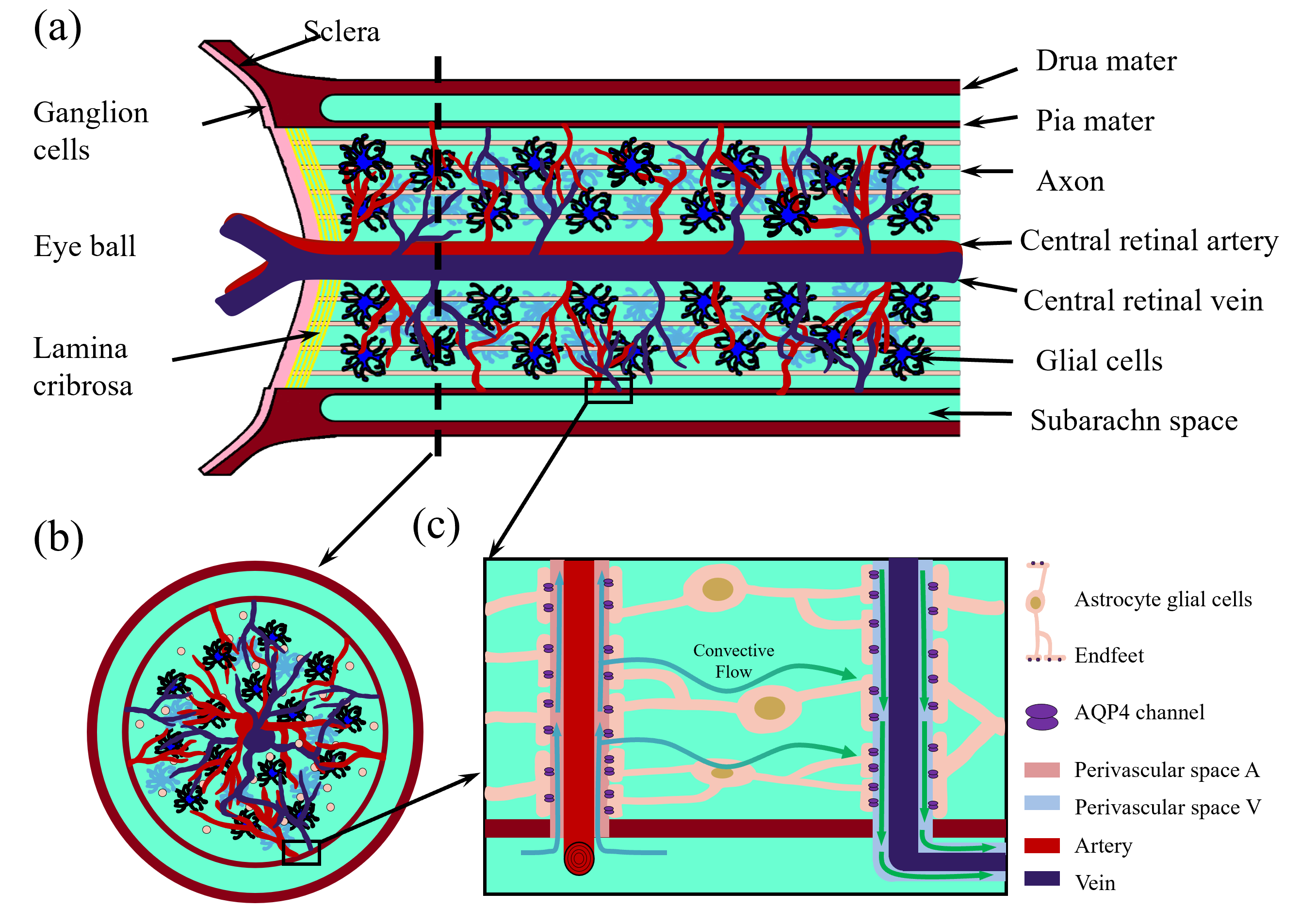 Fig. 1.
Optic nerve structure. (a) Longitudinal section of the optic nerve; (b) cross section of the optic nerve; (c) Local zoom in of the glymphatic system. This figure was drawn using MATLAB (R2023b, MathWorks, Inc., Natick, MA, USA).
For the optic nerve region, based on the model first proposed in Ref. [22], we
introduce a six-domain model for microcirculation of the optic nerve, which is
summarized in Table 1. We must remind the reader that the optic nerve bundler
contains many nerve fibers, at least one blood vessel, and a glial syncytium as
shown in Fig. 1. In addition to the axon (
| Compartment | Abbreviation | Subscription in formula |
| extracellular space | ECS | ex |
| perivascular space A | pvsA | pa |
| perivascular space C | pvsC | pc |
| perivascular space V | pvsV | pv |
| cerebrospinal fluid | CSF | csf |
| axon compartment | ax | ax |
| glial compartment | gl | gl |
ECS, extracellular space; CSF, cerebrospinal fluid.
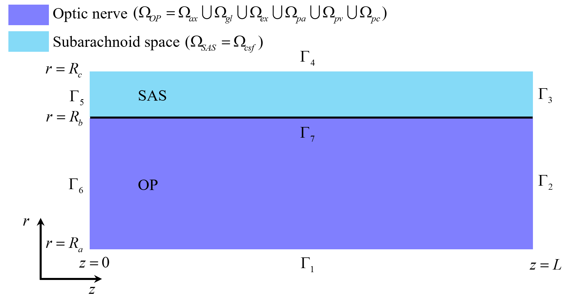 Fig. 2.
The optic nerve
We apply compartmental mass conservation laws to describe the dynamics of ions
and water within and across cellular and extracellular domains. These laws ensure
that the model respects fundamental physical principles—such as the
conservation of mass and charge—and establish a robust foundation for
physiologically realistic and numerically stable simulations. Specifically, the
model is derived from ion and fluid conservation laws governing transmembrane
transport between intracellular compartments and the ECS,
following the framework introduced in [24]. These conservation principles are
applied in each of the six domains:
where
For the boundaries,
In this model, the electric potential
Rather than solving the Poisson equation for
Based on the structure of the optic nerve, we have the following global assumptions for the model (Table 1).
where
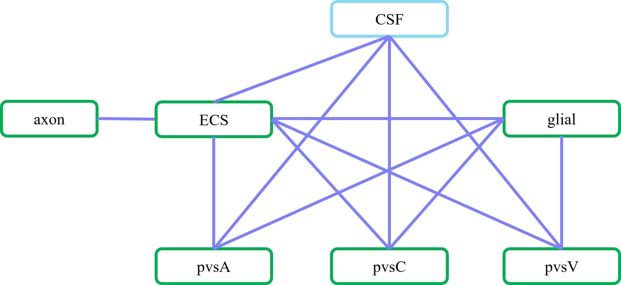 Fig. 3.
Schematic of communication between different compartments. In
the optic nerve
The details of the mathematical model can be found in the SI.
Our coupled ion and fluid transport model can be used for a wide range of studies. In this paper, we focus on the issue of potassium clearance in the optic nerve, leaving out many interesting questions to be explored in follow-up papers. In this section and the rest of our paper, we present simulation results and some discussions with the aim of understanding how glial cells and perivascular spaces facilitate potassium clearance during and after a train of stimulus.
As in Ref. [29], The model is solved using the Finite Volume Method on a uniform
mesh with axial symmetry, with equal discretization in the radial and axial
directions, i.e
All values of parameters are listed in Supplementary Table 1. Then, these resting-state values are used as initial conditions for the stimulus state.
Under a pressure gradient of 0.0083 mmHg/mm, CSF flows into the subarachnoid space (SAS) from the intracranial region,
with an average velocity of approximately 250 µm/s in the
z-direction, consistent with previous findings [31]. CSF then leaks into
perivascular space A. The flow direction in perivascular space A (or V) matches
the blood flow in the central retinal artery (or vein). The fluid flow in
perivascular space C adjusts dynamically through exchanges with other
compartments, primarily influenced by perivascular space V due to a larger
pressure gradient at boundary
In perivascular space A, the spatially averaged fluid velocity under a 0.007 mmHg/mm pressure gradient in the z-direction is 5 µm/s from the intracanalicular space to the intraorbital region. In perivascular space V, the spatially averaged fluid velocity in the z-direction under a –0.012 mmHg/mm pressure gradient is 4 µm/s from the intraorbital region to the intracanalicular space. These results align with the observations in [17, 32].
Simultaneously, fluid flows from pvsA into the ECS and the glial compartment through gaps and Aquaporin channels located near or on the glial cell feet [14], and then into perivascular space V. Fluid also moves from the ECS into the glial compartment, in agreement with the glymphatic system’s role [5, 13, 33].
This section examines the glymphatic system’s role (including glial cells and
perivascular spaces) in metabolic waste clearance during stimulation. As depicted
in Fig. 4, the stimulus is applied to the axon membrane within the region
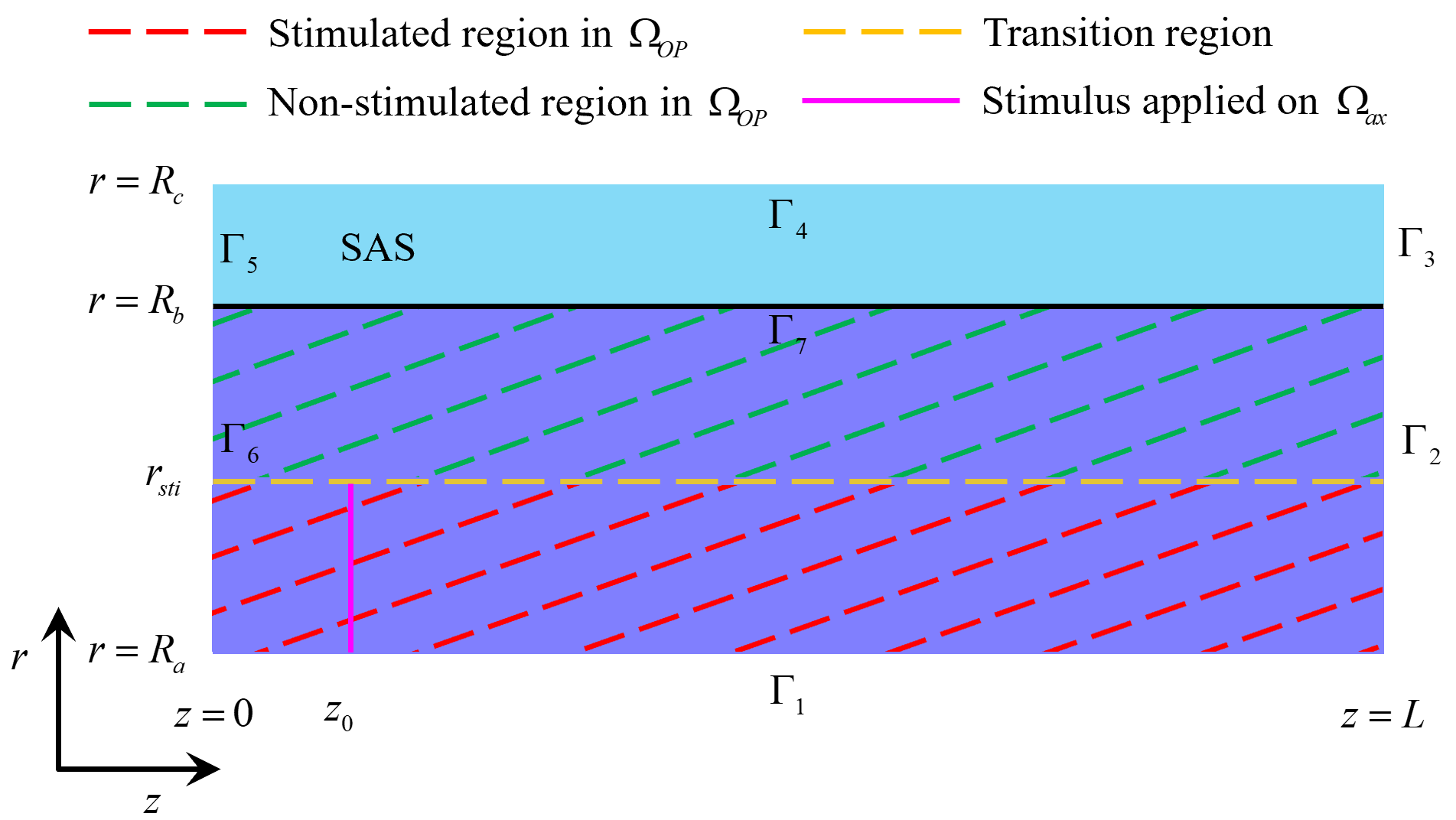 Fig. 4.
Stimulated and non-stimulated regions in the optic nerve
(
This section explores ionic circulation between stimulated and non-stimulated regions. During stimulation, as shown in Fig. 5a, Na+ ions enter the axon while K+ ions leak from the axon into the ECS (see Fig. 5i), leading to potassium accumulation in the stimulated region. Snapshots of potassium concentration in the ECS, shown in Fig. 6, indicate that potassium concentration initially rises in the stimulated region, reaching up to 5.3 mM. Subsequently, through the buffering function of the glymphatic system, the accumulated potassium is transported from the stimulated to the non-stimulated region, lowering the overall concentration in the optic nerve to 4.9 mM.
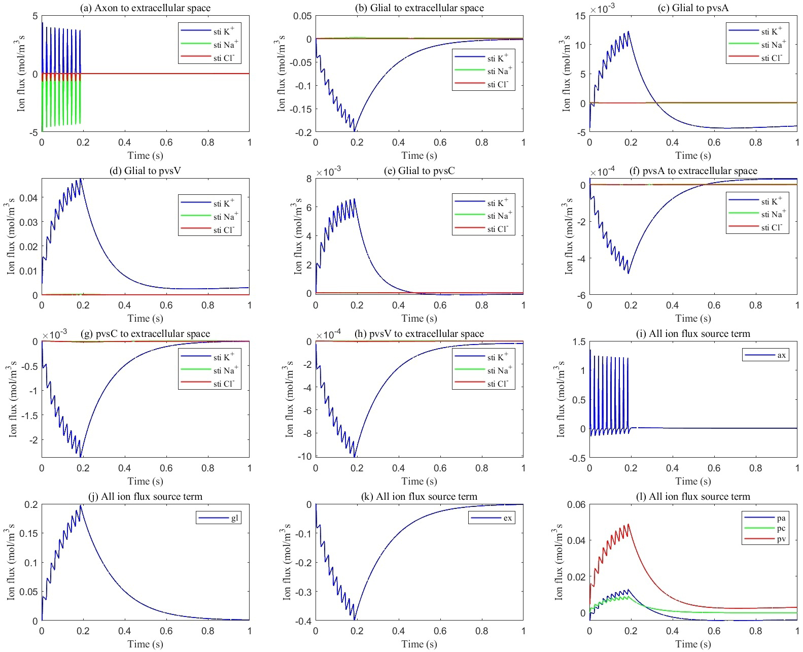 Fig. 5.
Average transmembrane ion flux in the stimulated region. (a) from axon to ECS; (b) from glia to ECS; (c) from glia to pvsA; (d) from glia to pvsV; (e) from glia to pvsC; (f) from pvsA to ECS; (g) from pvsC to ECS; (h) from pvsV to ECS; (i) total ion flux flows into axon; (j) total ion flux flows into glia; (k) total ion flux flows into ECS; (l) total ion flux flows into pvs.
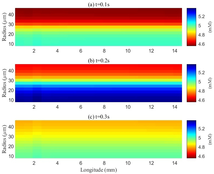 Fig. 6.
Spatial distribution of potassium concentration in the extracellular space (ECS) during and after a train of stimuli. a, b, and c represent the spatial distribution of potassium ions at different time points: 0.1 s, 0.2 s, and 0.3 s, respectively. The initial potassium concentration in the ECS was 4.5 mM. Upon electrical stimulation of the axons, action potentials were generated, resulting in potassium efflux into the ECS and a localized increase in potassium concentration within the stimulated (lower) region. The potassium concentration in this area peaked at 5.3 mM by the end of the stimulation period (0.2 s). During stimulation, excess potassium also diffused from the stimulated region into adjacent non-stimulated regions. After the cessation of stimulation, the potassium concentration gradually re-equilibrated throughout the ECS.
Fig. 7a illustrates three mechanisms for buffering the accumulated potassium: the glial compartment, the perivascular space, and diffusion within the ECS. Fig. 7b illustrates the potassium spatial buffering and water circulation between ECS and glial compartment. The interaction between osmotic pressure difference, convection, diffusion, and electrical drift is demonstrated in detail.
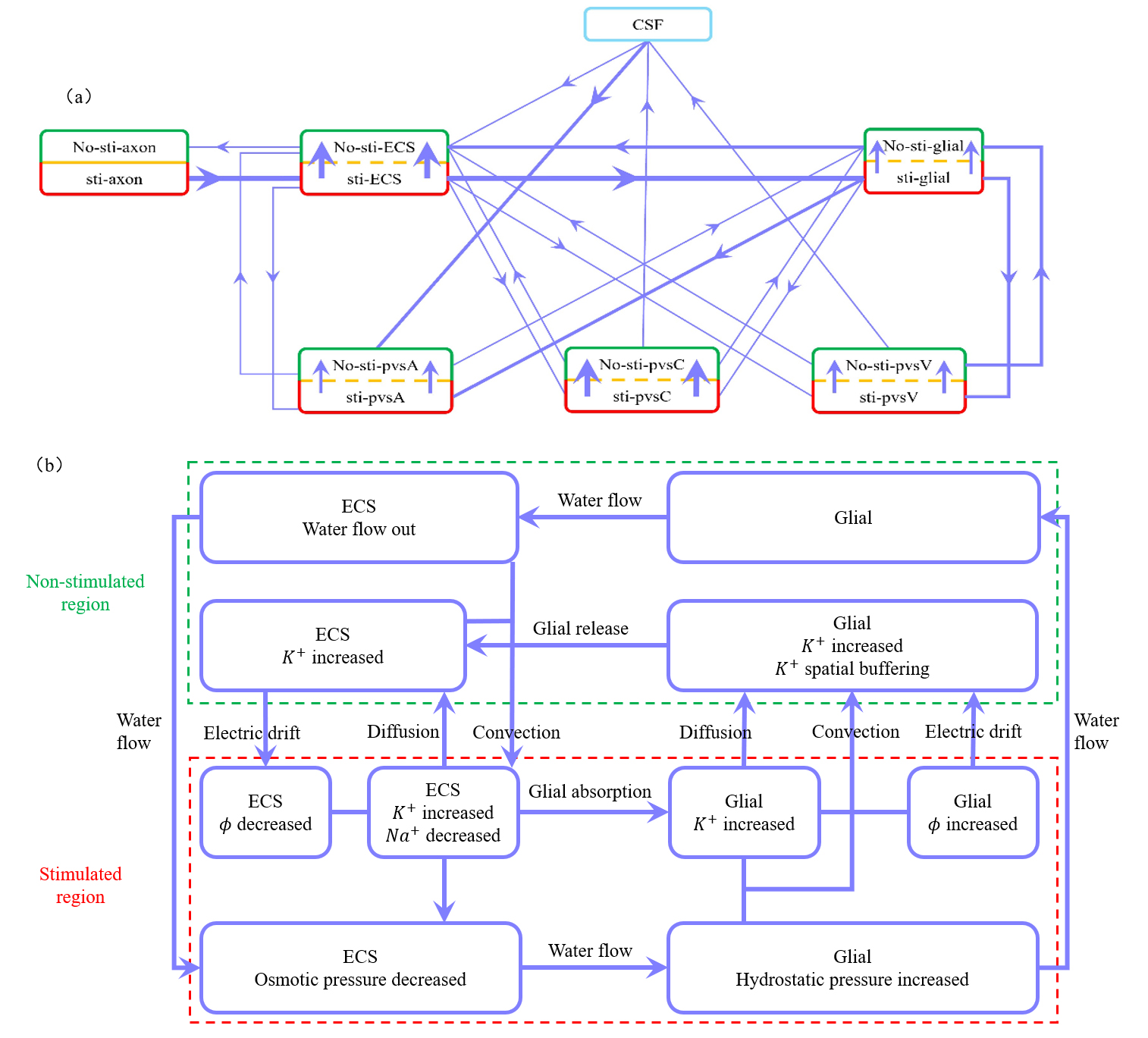 Fig. 7.
Illustration of microcirculation and the roles of diffusion, convection and electric drift. (a) Schematic of potassium flux between the stimulated (lower) and non-stimulated (upper) regions, as well as transmembrane flux between different compartments during stimulation. Red boxes represent stimulated regions, and green boxes represent non-stimulated regions. The thickest lines indicate fluxes around 10-1 mol/(m3s), moderately thick lines represent fluxes around 10-2 mol/(m3s), and the thinnest lines indicate fluxes less than 10-3 mol/(m3s). (b) Schematic description for potassium spatial buffering and water circulation between ECS and glial compartment. When axon is stimulated to release an action potential, potassium ions flow out while sodium ions flow in, leading to an increase potassium concentration and a decrease in osmotic pressure in ECS. In the stimulated region, potassium ions enter glial from the ECS through the glial membrane, raising the electrical potential in the glial compartment. The water flow out of ECS into glial with the osmotic pressure different. Within the glial compartment, the hydrostatic pressure and the potassium concentration are increased in stimulated region. The water flow from the stimulated region into the non-stimulated region. And the potassium diffusion, convection, electric drift are all causing potassium to flow from the stimulated region to the non-stimulated region. But the electric drift dominates. In the non-stimulated region, potassium leak back into the ECS by flowing out of the glial through the glial membrane. And due to the osmotic pressure difference, water flows from the glial compartment back into the ECS. Within the ECS, potassium carried by water convection and electric drift from the non-stimulated region back to the stimulated region, while diffusion dominates, causing potassium to flow from the stimulated region to the non-stimulated region. the hydrostatic pressure difference drives water to flow back from the non-stimulated region to the stimulated region, completing the cycle. This figure was drawn using MATLAB (R2023b, MathWorks, Inc., Natick, MA, USA).
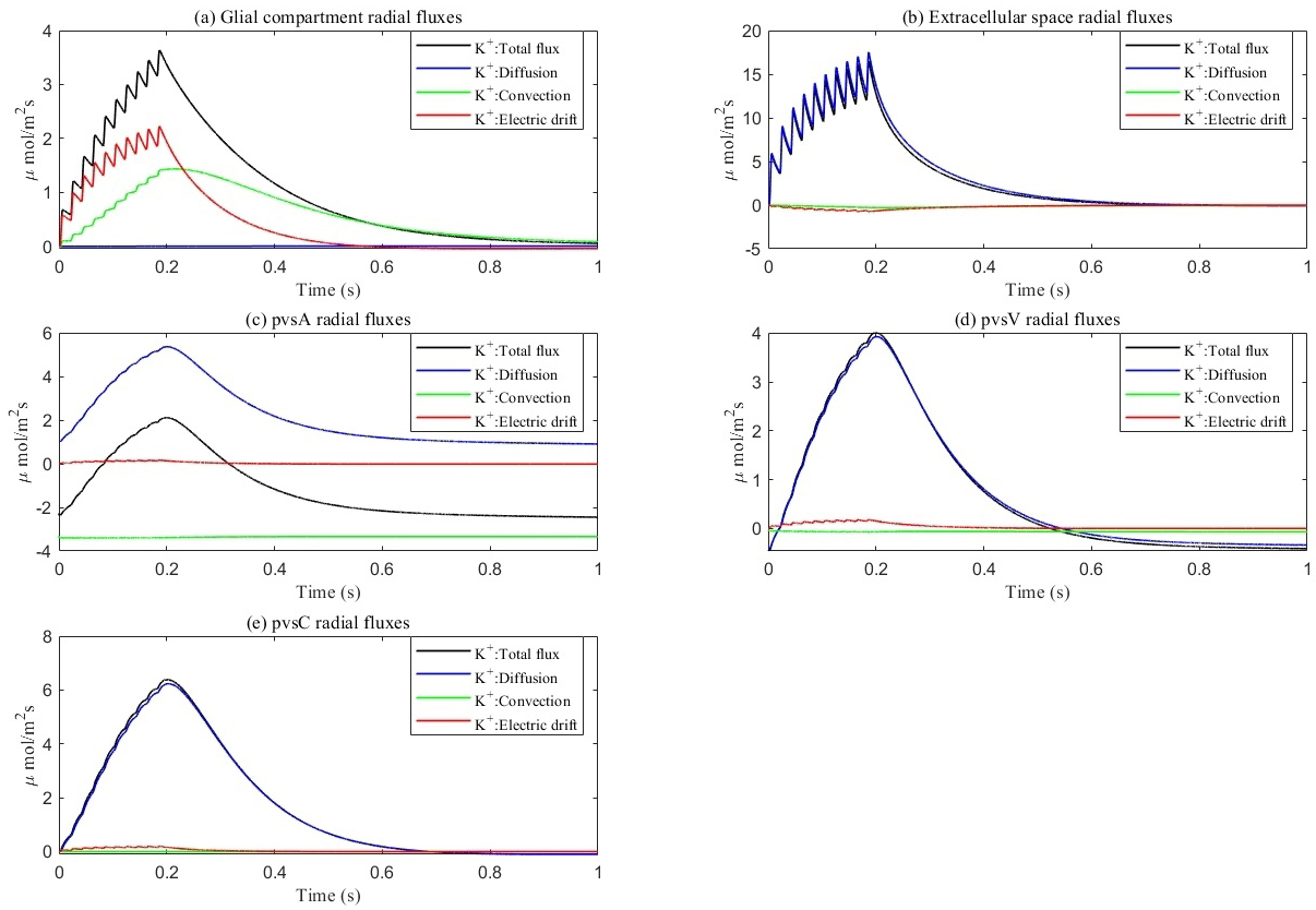 Fig. 8.
Average radial direction potassium flux components within each compartment. (a–e) represent different components, respectively. (a) glial compartment. (b) ECS. (c) pvsA. (d) pvsV. (e) pvsC. Total flux equals diffusion flux plus convection flux plus electric drift flux. In glial compartment, the electric drift is dominant. In ECS and PVS, the diffusion is dominant.
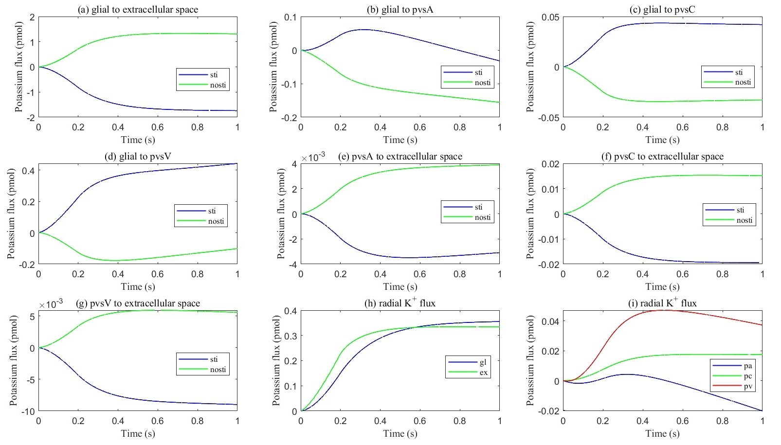 Fig. 9.
Cumulative transmembrane flux between different comparts. (a–g) Cumulative transmembrane potassium fluxes in the stimulated and non-stimulated regions after neuronal firing stops. (h,i) Radial cumulative potassium fluxes within compartments after neuronal firing stops.
A detailed illustration of potassium microcirculation between the different compartments is available in Supplementary material Fig. 1. And the sodium flux inside each domain can be found in Supplementary material Fig. 3.
Fig. 9 presents the cumulative potassium flux (total potassium flux integrated over time). The results indicate that the cumulative potassium flux through the glial membrane is twice as large as the radial cumulative potassium flux inside the ECS, two orders of magnitude larger than in pvsC, and three orders of magnitude larger than in pvsA and pvsV within the stimulated ECS. Concurrently, the cumulative potassium flux through the glial membrane into pvsV is 1.5 times the radial cumulative potassium flux inside the glial membrane and an order of magnitude larger than in pvsA and pvsC within the stimulated glial compartment during a train of stimuli.
In summary, these numerical results confirm that the glial compartment is the most critical and rapid pathway for potassium transport, while the perivascular spaces provide secondary pathways for potassium removal from the stimulated region when neurons fire or stop firing. Over time, potassium circulation and concentrations in each compartment return to the resting state.
While this paper primarily focuses on potassium clearance, we provide a brief summary of fluid circulation in Supplementary material Fig. 2, with further details to be explored in a separate paper. Fluid circulation during and after stimulation is driven by two primary forces: hydrostatic pressure differences and osmotic pressure differences. See Fig. 5i–l, the selective permeability of the cell membrane to different ions leads to variations in osmotic pressure between different components. Hydrostatic pressure gradients within the subarachnoid space (SAS) and perivascular spaces direct the movement of CSF and interstitial fluid through the optic nerve compartments. Simultaneously, osmotic pressure, influenced by ionic microcirculation, drives fluid exchange between the ECS, glial compartments, and perivascular spaces. These mechanisms work together to facilitate fluid redistribution, ensuring efficient clearance of metabolic waste and maintaining homeostasis between the stimulated and non-stimulated regions. The dynamic interaction between these forces allows fluid circulation to adapt in response to neuronal activity, supporting the glymphatic system’s overall function in the optic nerve.
In this section, we investigate the role of the glial compartment in
extracellular potassium buffering by varying the transmembrane ionic conductance
(
Research suggests that in neurodegenerative diseases, oxidative stress and
inflammation can impair ion channels on astrocytes, reducing their conductivity
[34, 35]. To simulate these effects, we reduced the membrane conductivity to
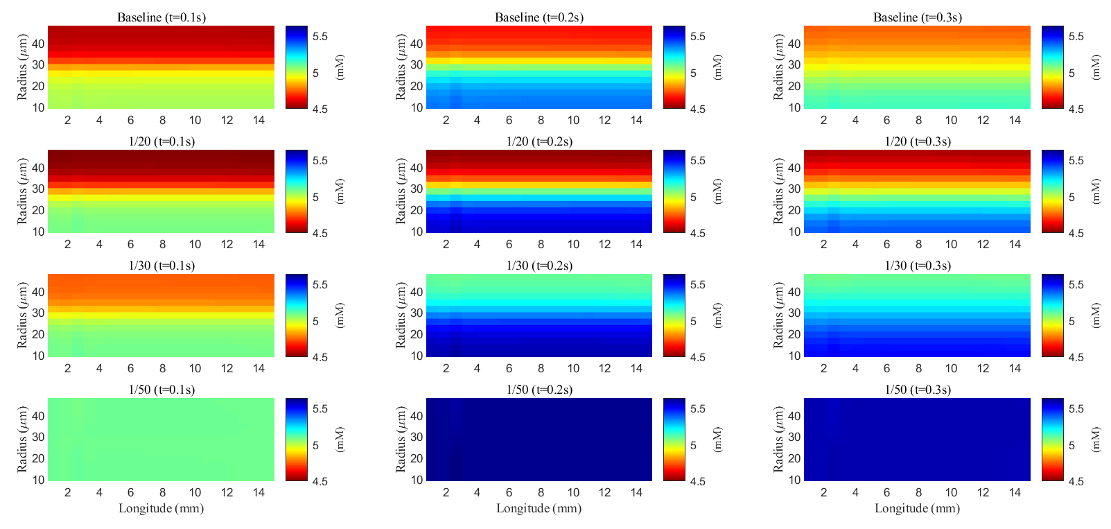 Fig. 10.
Spatial distribution of potassium concentration during and after a train of stimuli in the ECS. Different rows are results with different membrane conductance; Different columns are results at different time slots.
As glial membrane conductance decreases, the transmembrane flux through the
glial compartment is reduced (see Fig. 11c–f), resulting in less efficient
potassium clearance from the ECS (see Fig. 11a). When the conductance is reduced
to
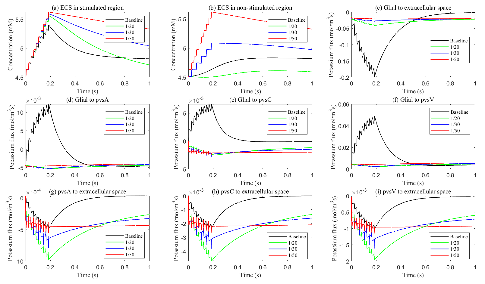 Fig. 11.
Potassium concentration and transmembrane potassium flux with different glial membrane conductance. (a,b) The potassium concentration in the stimulated and non-stimulated regions. (c–i) The transmembrane potassium flux in stimulated region.
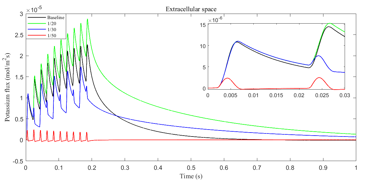 Fig. 12.
Average radial potassium flux within the ECS with different glial membrane conductance. The subplot shows the radial potassium flux during a single action potential.
The role of the glial compartment is not limited to potassium buffering. Fig. 13
shows the results during the first stimulus. We applied the same stimulation
protocol. The stimulus region showed minimal variation in axonal membrane
potential. See Fig. 13c. At the onset of stimulation, the field potential in the
extracellular region decreases (see Fig. 13a) as Na+ channels activate,
allowing more Na+ to enter the axon. This raises the axonal potential and
causes potassium to leak out of the glial compartment because the transmembrane
potential (
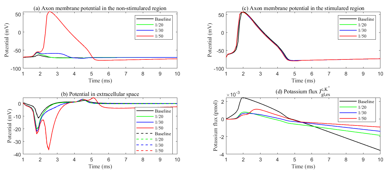 Fig. 13.
Membrane potential with different membrane conductance. (a) Axon membrane potential in the non-stimulated region. (b) The electric potential in the ECS in the stimulated region (solid line) and non-stimulated region (dash line). (c) Axon membrane potential in the stimulated region. (d) The cumulative potassium flux through the passive ion channel on the glial membrane from the glial compartment to the ECS. Different lines mean different glial membrane conductance. During sustained stimulation, potassium flux from glial to the ECS maintains ECS potential within physiological range, thereby preventing passive action potential generation in non-stimulated regions.
During the later stages of the action potential, K+ channels are activated,
and more K+ ions enter the ECS, making the Nernst potential
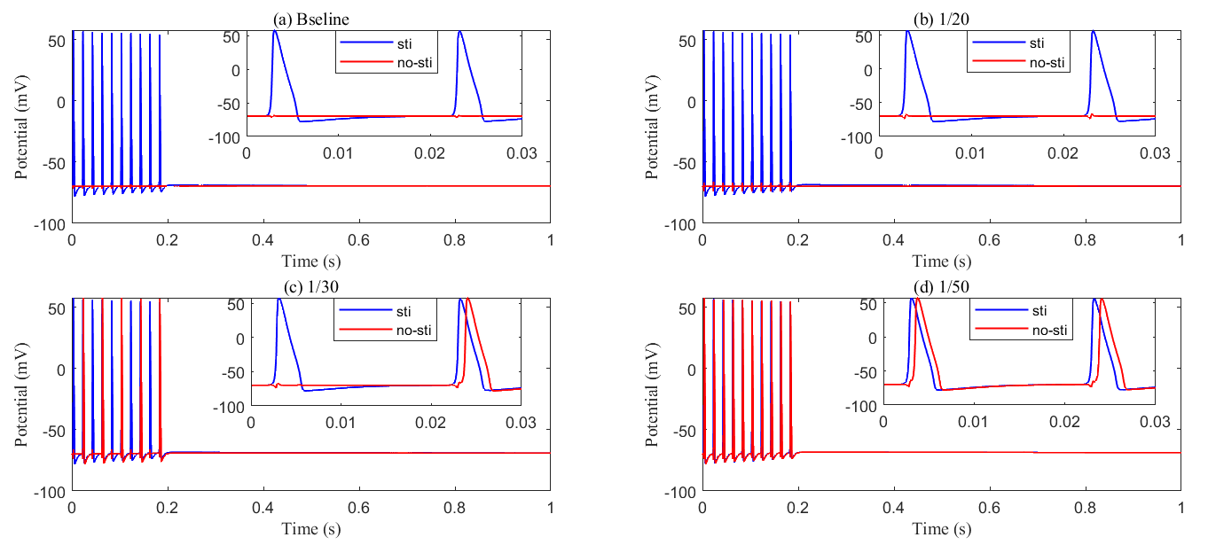 Fig. 14.
Recording axon membrane potential in the stimulated (blue) and non-stimulated (red) region with different glial membrane conductance. (a) Baseline results; (b) conductance reduced to be 1/20 of baseline; (c) conductance reduced to be 1/30 of baseline; (d) conductance reduced to be 1/50 of baseline. As the membrane conductance of glial cells decreases, abnormal axonal firing occurs, generating passive action potentials in non-stimulated regions.
In summary, glial cell ionic conductivity, particularly involving potassium regulation, is crucial for preventing neuronal hyperexcitability and the development of epilepsy. Dysfunction in these mechanisms can lead to disrupted ionic homeostasis, contributing to the occurrence of seizures.
Connexins in glial cells, particularly astrocytes, form gap junctions that
facilitate direct communication between cells by allowing the passage of ions,
small molecules, and signaling substances. These connexins play a crucial role in
maintaining ionic balance, including potassium clearance in the brain’s ECS.
However, in certain pathological conditions or through experimental
interventions, connexin function can be disrupted or blocked [37]. Such
dysfunction reduces the connectivity of the glial compartment. In our simulation,
we decrease the diffusion coefficients
After a stimulus, potassium, and fluid flow from the extracellular space into
the glial compartment due to differences in Nernst potential and osmotic
pressure. Fig. 15 shows the spatial distribution of electric potential within the
glial compartment (long-term behavior can be found in Supplementary material Fig. 4). As
connexin connectivity decreases, the intracellular conductance
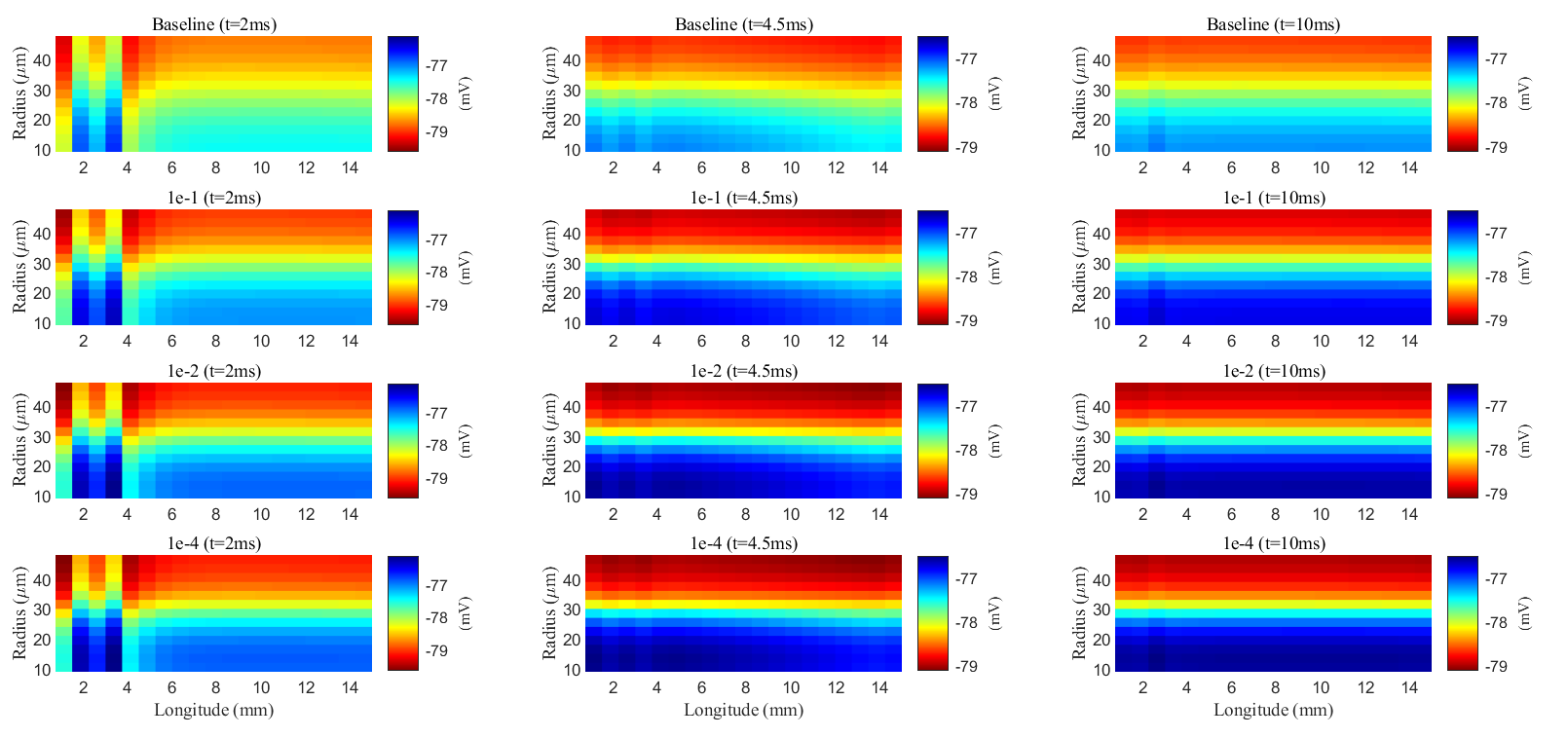 Fig. 15.
Spatial distribution of membrane potential during a stimulus in the glial compartment. Different rows are results with different connectivity of glial compartments. Different columns are results at different time slots.
Although potassium concentration remains nearly constant (see Fig. 16), due to the swelling of the glial compartment, the rising glial membrane potential (see Fig. 16b) reduces the transmembrane potassium influx, as shown in Fig. 17f. The reduction in permeability and diffusion within the glial compartment leads to a significant decrease in the potassium buffering flux (see Fig. 17a). In this scenario, the glial compartment in the stimulated region acts as a reservoir, absorbing excess potassium and protecting the axonal cells.
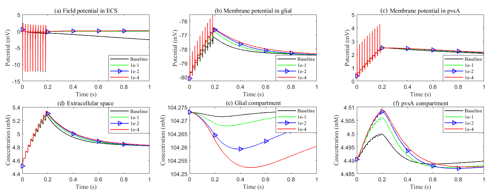 Fig. 16.
Effects of glial connexin connectivity on the membrane potential and potassium clearance. (a–c) Field potential and membrane potential in the stimulated region. (d–f) Potassium concentration in the stimulated region.
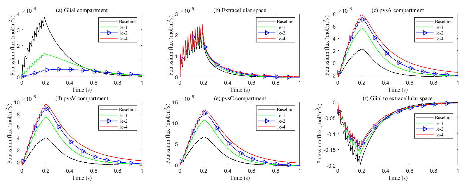 Fig. 17.
Effects of glial connexin connectivity on the transmembrane potassium flux. (a–e) Average radial potassium flux in the intradomain with varying levels of glial connexin connectivity. (f) Average transmembrane potassium flux from glial to ECS in the stimulated region.
At the same time, the elevated electric potential in the glial compartment enhances the flux from the glial compartment to the perivascular spaces (see Fig. 18a–c), increasing the intra-compartment flux within the perivascular space (see Fig. 17c–e). The reduced permeability within glial compartment enhances the flow of potassium ions from the ECS to the pvs (see in Fig. 18d–f), while the radial potassium flux in the extracellular space exhibits a slight but insignificant increase (see in Fig. 17b). This suggests that the perivascular spaces take on a more prominent role in buffering potassium in these conditions (see Figs. 5,6 in Supplementary material). However, compared to the glial electric drift mechanism, convection-based transport in the perivascular spaces is less efficient for potassium clearance (see Fig. 16d).
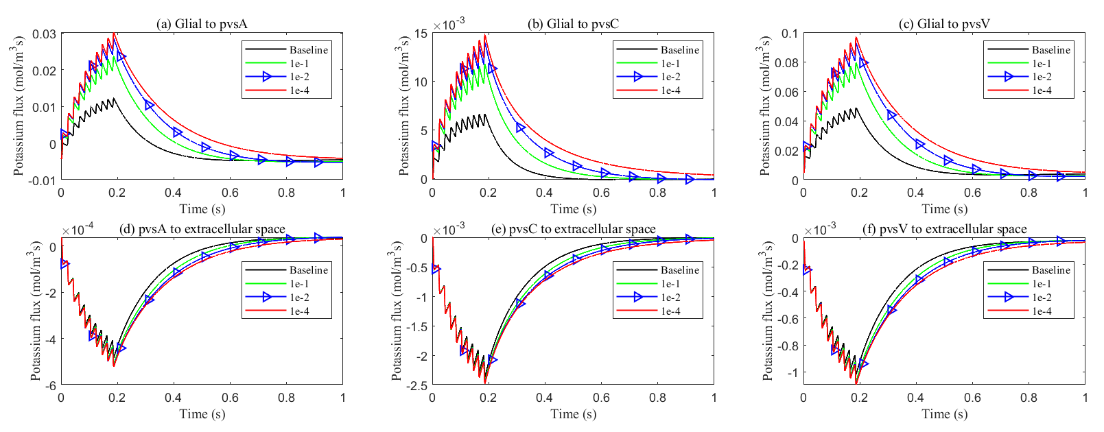 Fig. 18.
Average transmembrane potassium flux on perivascular spaces with varying levels of glial connexin cnnectivity in the stimulated region. Transmembrane K+ fluxes (a) from glia to pvsA; (b) from glia to pvsC; (c) from glia to pvsV; (d) from pvsA to ECS; (e) from pvsC to ECS; (f) from pvsV to ECS.
In summary, the glial pathway is the most important mechanism for potassium buffering and clearance, while the perivascular space pathway serves as the second most important. When the pathways of glial compartment are compromised, whether it is the glial membrane or the internal pathways of the glial compartment, the perivascular space pathway takes on a more significant role in buffering potassium ions from the ECS.
This study presents a multicompartment model of the optic nerve that integrates ionic electrodiffusion, osmotic water transport, and convective fluid flow across axons, glial cells, the ECS, and perivascular domains. By extending earlier frameworks, we incorporate glial–vascular interactions to investigate potassium buffering and clearance following neuronal stimulation.
Our simulations demonstrate that potassium released from axons during activation accumulates in the ECS and is rapidly cleared through two major pathways: (i) uptake by glial cells, and (ii) fluid-mediated redistribution via perivascular spaces. The efficiency of this clearance strongly depends on glial membrane conductance and intercellular connexin permeability. Reduced glial conductance leads to ectopic neuronal excitation, resembling epileptic activity, while impaired gap junction connectivity increases reliance on perivascular drainage. These results highlight the cooperative role of glia and vasculature in maintaining extracellular ionic homeostasis. The model reveals that potassium transport is primarily driven by electric drift within glial syncytia, while osmotic and convective forces regulate fluid movement. This interaction enables volume preservation and ion redistribution under varying physiological conditions.
While our model provides valuable insights, it has several limitations that could be addressed in future studies:
Despite these limitations, our model is inherently designed to describe multidomain coupling in central nervous system (CNS) microcirculation, where ionic electrodiffusion, fluid flow, and cellular compartmentalization are tightly integrated. It is particularly well-suited for structures with approximately cylindrical geometry, such as the optic nerve. However, when applying this model to other neural structures with significantly different geometries—such as the retina, which has a hemispherical shape—modifications would be necessary. For instance, the assumption of axial symmetry may no longer hold, and the geometry would need to be reparametrized accordingly. One approach is to introduce a deformation or curvature parameter that adjusts the radial coordinate as a function of axial distance, allowing the model to approximate a curved domain while preserving numerical efficiency. In addition, cell types and their layout also need to be taken into consideration.
In addition, different tissue types may involve distinct membrane surface areas, permeability profiles, and ion channel distributions. These physiological differences can be incorporated into the current framework by adjusting the relevant coefficients and source terms, without altering the underlying mathematical structure. Although the model does not explicitly resolve fine-scale anatomical heterogeneity, it captures emergent spatial variation in compartmental volume fractions driven by fluid transport. This coarse-grained approach offers a practical and physiologically meaningful basis for system-level investigations. In future work, we plan to refine the model by incorporating spatially varying parameters—such as ion pump density and vascular architecture—or by integrating image-derived geometries to simulate region-specific dynamics under both healthy and pathological conditions.
Moreover, this model holds significant potential for simulating pathological conditions such as epilepsy, in which disrupted ion homeostasis, impaired fluid dynamics, and compromised clearance mechanisms contribute to disease progression. The insights gained from our simulations—such as abnormal potassium accumulation and ectopic axonal excitation in response to altered glial ion permeability—can help identify key physiological thresholds and failure points. These findings may inform the development of therapeutic strategies aimed at modulating glial function or enhancing solute clearance via perivascular pathways, ultimately supporting neuronal stability and resilience.
The datasets used and analyzed during the current study are available from the corresponding author on reasonable request.
HH, SX and RE conceived and designed the research study. SFX conducted the research. SFX, HH, ZS, and SX contributed to model development. SFX, ZS, and SX implemented the computational programming. SFX, RE, and SX drafted and revised the manuscript. All authors contributed to editorial changes in the manuscript. All authors read and approved the final manuscript. All authors have participated sufficiently in the work and agreed to be accountable for all aspects of the work.
Not applicable.
Not applicable.
This work was partially supported by the National Natural Science Foundation of China no.12231004 (H. Huang) and 12071190 (S. Xu).
The authors declare no conflict of interest.
During the preparation of this work, the authors used ChatGPT to improve the language and readability. After using this tool/service, the authors reviewed and edited the content as needed and take full responsibility for the content of the published article.
Supplementary material associated with this article can be found, in the online version, at https://doi.org/10.31083/FBL39722.
References
Publisher’s Note: IMR Press stays neutral with regard to jurisdictional claims in published maps and institutional affiliations.