This retrospective study was conducted at the First Hospital of Lanzhou University in Gansu Province, spanning from January 1, 2019, to December 31, 2020. The study included all consecutive hospitalized patients diagnosed with AMI who received PCI. The diagnosis of AMI was established in accordance with the European Society of Cardiology Guidelines [2]. The inclusion criteria were as follows: (1) a confirmed diagnosis of AMI, (2) age $\ge$18 years, (3) patients who underwent PCI, and (4) availability of complete clinical information. The inclusion and exclusion processes are illustrated in Fig. 1. Initially, 1801 patients were identified; however, 53 were excluded due to significant missing data, 38 due to misdiagnoses, and 17 because they did not undergo PCI. Ultimately, 1693 patients were included for further analysis.

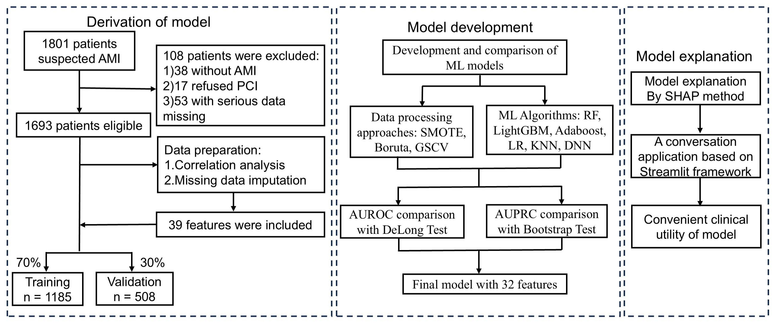Fig. 1.

Flowchart of AMI patient inclusion and exclusion, and the ML model development process. AMI, acute myocardial infarction; PCI, percutaneous coronary intervention; ML, machine learning; SMOTE, synthetic minority over-sampling technique; GSCV, grid search with cross-validation; SHAP, shapley additive explanation; AUROC, area under the receiver operating characteristic curve; AUPRC, area under the precision-recall curve; RF, Random Forest; LightGBM, Light Gradient Boosting Machine; AdaBoost, Adaptive Boosting; LR, Logistic Regression; KNN, K-Nearest, Neighbors; DNN, Deep Neural Networks.

Clinical and laboratory data for patients with AMI were extracted from electronic medical records, with a particular focus on IHM. The relevant laboratory tests and clinical data are summarized in Table 1. The results of the initial laboratory test conducted upon hospital admission prior to PCI were recorded, along with the corresponding blood sample data. To manage missing data, two approaches were employed: features with more than 20% missing data were excluded, while for those with less than 20% missing data, the IterativeImputer method was utilized to minimize bias. Based on parameters from established risk scores (e.g., GRACE, TIMI) and the latest guideline-based insights into AMI pathophysiology, supplemented by input from clinical experts, we identified 39 potential prognostic variables for AMI outcomes [1, 3, 5]. These variables, encompassing demographic information, cardiovascular history, and laboratory indicators, were incorporated into the analysis. Specifically, the variables included gender, age, total ischemia time (TIT), type 2 diabetes mellitus (T2DM), hypertension (HTN), hyperlipidemia (HLD), peripheral artery disease (PAD), smoking history (SH), coronary artery disease (CAD), bleeding history (HB), body mass index (BMI), systolic blood pressure (SBP), diastolic blood pressure (DBP), heart rate (HR), creatinine (CREA), uric acid (UA), random blood glucose (RBG), low-density lipoprotein cholesterol (LDL-C), estimated glomerular filtration rate (eGFR), hematocrit (HCT), neutrophil count (NEUT), lymphocyte count (LYMPH), neutrophil-to-lymphocyte ratio (NLR), hemoglobin (HGB), platelet count (PLT), C-reactive protein (CRP), myoglobin (MYO), creatine kinase–myocardial band (CK-MB), troponin I (TNI), N-terminal pro–B-type natriuretic peptide (NT-proBNP), hemoglobin A1c (HbA1c), left atrial diameter (LAD), left ventricular ejection fraction (LVEF), left ventricular end-diastolic volume (LVEDV), left ventricular end-systolic volume (LVESV), MB, ventricular fibrillation (VF), atrial fibrillation (AF), and cardiogenic shock (CS).

In this study, CAD was defined as the presence of $\ge$50% stenosis, prior revascularization, or a history of MI. MB was characterized by a hemoglobin drop of $\ge$3 g/dL or the transfusion of $\ge$2 units of blood. CS was diagnosed based on a SBP of less than 90 mmHg persisting for over 30 minutes, the necessity for vasopressors or mechanical support, evidence of hypoperfusion, or classification as Killip class IV. HB was defined as any clinically significant bleeding occurring within the previous 12 months.

Patients were randomly divided into training and testing cohorts in a 70:30 ratio. Three data processing techniques were employed: Synthetic Minority Over-sampling Technique (SMOTE) to address class imbalance [16, 17, 18], Boruta for feature selection [19], and Grid Search with Cross-Validation (GSCV) for hyperparameter tuning [20]. Six ML algorithms were evaluated: Random Forest (RF), Light Gradient Boosting Machine (LightGBM), Adaptive Boosting (AdaBoost), Logistic Regression (LR), K-Nearest Neighbors (KNN), and Deep Neural Networks (DNN).

Model development adhered to a structured framework: (1) identifying optimal processing methods, (2) selecting the best-performing algorithm, and (3) constructing the final predictive model by integrating the chosen strategies (Fig. 1). Model performance was primarily assessed using the AUROC and AUPRC [21], while secondary metrics such as accuracy, precision, sensitivity, specificity, and F1-score supported model selection. To enhance interpretability, SHAP values were employed to assess feature importance and quantify each variable’s contribution to the model’s predictions.

Baseline characteristics between the survival and mortality groups were compared. For normally distributed data, the Independent Samples t-test was employed, with results expressed as the mean $\pm$ standard deviation. For non-normally distributed data, the Mann–Whitney U test was utilized, and results were presented as the median $\pm$ interquartile range. DeLong’s test was conducted to compare AUROC differences between models, while the Bootstrap test assessed differences in AUPRC. Categorical variables were analyzed using the Chi-Squared test. All statistical analyses were performed using R 4.3.1 software (R Foundation for Statistical Computing, Vienna, Austria), whereas ML algorithms, including BorutaShap, SHAP, AUROC, and AUPRC, were implemented using Python 3.11.9 software (Python Software Foundation, Wilmington, DE, USA). A two-tailed p-value of 0.05 was deemed statistically significant.

This prospective study included 1693 patients in the derivation cohort for the development of the IHM prediction model. Among these patients, 34 (2.0%) died in-hospital following PCI. A detailed comparison of demographic and clinical variables among the training, testing, survived, and deceased cohorts is provided in Table 1.

The first phase centered on optimizing data processing while consistently employing the RF algorithm. This process sequentially applied the SMOTE for class balancing, GSCV for hyperparameter tuning, and the Boruta algorithm for feature selection, with the aim of identifying the most effective processing strategy. Model performance was assessed using the AUROC and the AUPRC, as illustrated in Fig. 2A,B.

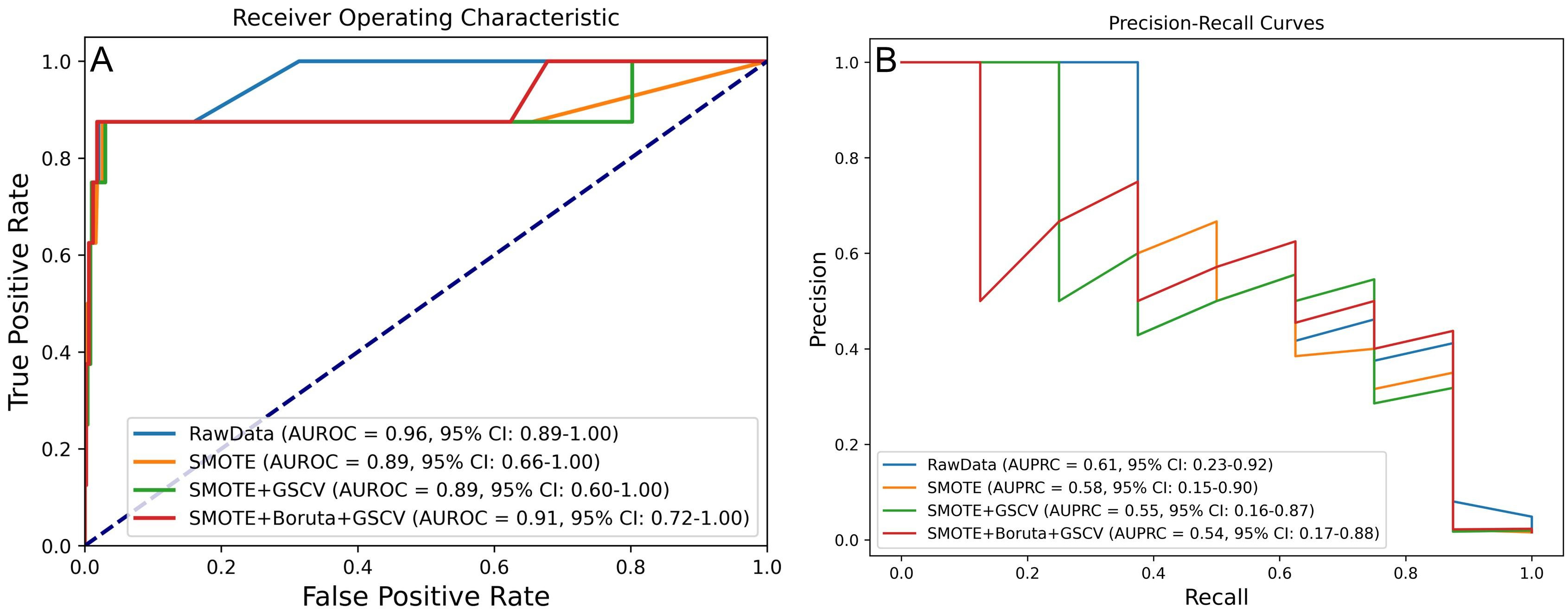Fig. 2.

Model performance under four processing strategies for predicting IHM in AMI patients post-PCI. (A) AUROC and (B) AUPRC values across different processing levels. IHM, in-hospital mortality.

DeLong and bootstrap tests were employed to compare the AUROC and the AUPRC across various processing strategies (Supplementary Fig. 1). The results indicated no statistically significant differences (p $>$ 0.05), suggesting that the processing method alone did not substantially impact model performance. Consequently, model selection was guided by secondary metrics and a preference for simpler models. For the model trained using SMOTE, Boruta, and GSCV, the validation set yielded an AUROC of 0.91 (95% CI: 0.72–1.00) and an AUPRC of 0.54 (95% CI: 0.17–0.88).

Additional metrics, including accuracy, precision, sensitivity, specificity, and F1 score, were utilized for model evaluation. As summarized in Table 2, the model trained with SMOTE and GSCV achieved the best overall performance, with an AUROC of 0.892, accuracy of 0.986, precision of 0.556, sensitivity of 0.625, specificity of 0.992, and an F1 score of 0.588.

The second phase aimed to identify the optimal ML algorithm using the previously determined best processing strategy. Six algorithms were evaluated, with the results of AUROC and AUPRC presented in Fig. 3A,B. Among these, RF, LightGBM, and LR demonstrated superior predictive performance. Specifically, RF achieved an AUROC of 0.95 (95% CI: 0.84–1.00) and an AUPRC of 0.57 (95% CI: 0.17–0.90); LightGBM reached an AUROC of 0.96 (95% CI: 0.86–1.00) and an AUPRC of 0.52 (95% CI: 0.17–0.97); LR recorded an AUROC of 0.97 (95% CI: 0.91–1.00) and an AUPRC of 0.56 (95% CI: 0.15–0.88).

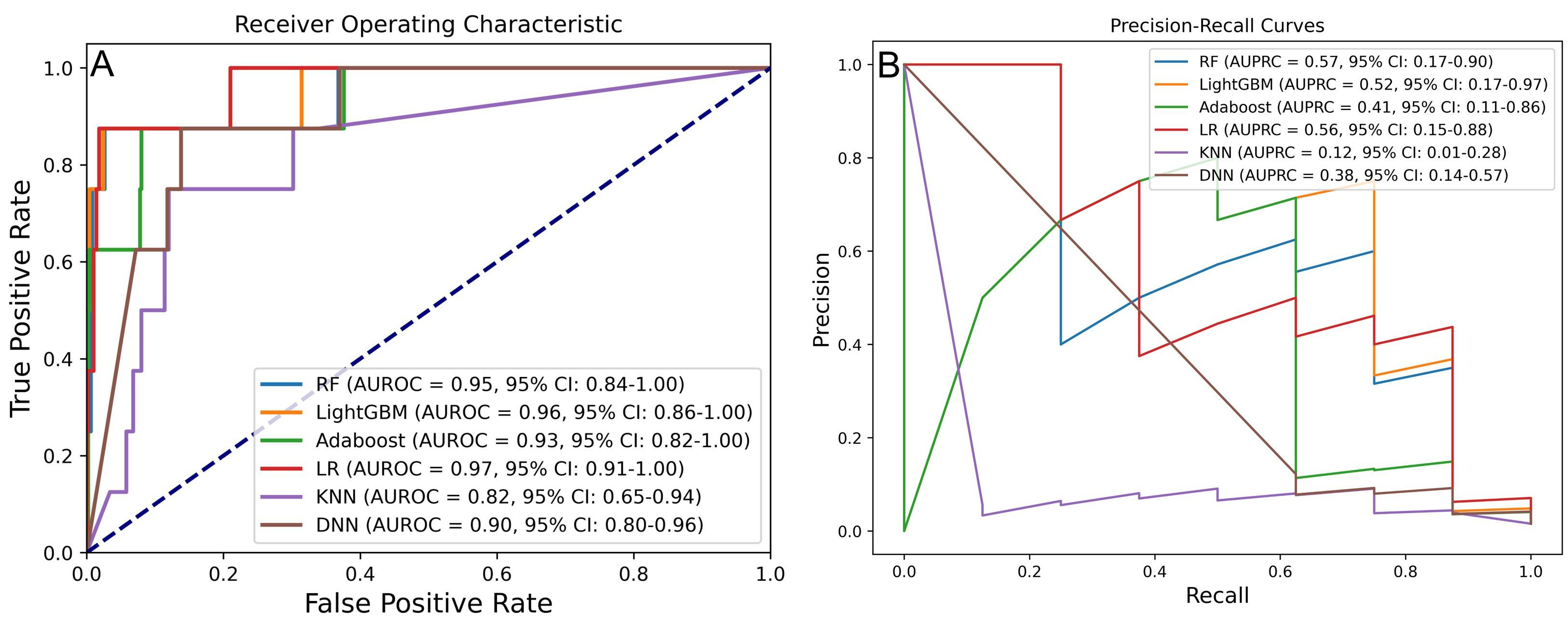Fig. 3.

Performance comparison of six ML models for predicting IHM in AMI post-PCI. (A) AUROC and (B) AUPRC for models developed with different algorithms. RF, random forest; LightGBM, light gradient boosting machine; AdaBoost, adaptive boosting; LR, logistic regression; KNN, k-nearest neighbor; DNN, deep neural network.

DeLong and bootstrap tests were performed to compare AUROC and AUPRC differences across models (Supplementary Fig. 2). While the AUROC differences were not statistically significant (p $>$ 0.05), RF and LightGBM significantly outperformed KNN in terms of AUPRC (p 0.05).

Model evaluation using additional metrics—including accuracy, precision, sensitivity, specificity, and F1 score—further supported RF and LightGBM as the top-performing models. As shown in Table 3, RF achieved an AUROC of 0.948, an accuracy of 0.988, a precision of 0.625, a sensitivity of 0.625, a specificity of 0.994, and an F1 score of 0.625. LightGBM achieved an AUROC of 0.956, an accuracy of 0.992, a precision of 0.750, a sensitivity of 0.750, a specificity of 0.996, and an F1 score of 0.750.

In the final model selection phase, the RF model, trained using SMOTE, Boruta, GSCV, and RF, was selected as the primary option. The LightGBM1 model, which utilized SMOTE, Boruta, GSCV, and LightGBM, was chosen as the secondary option, followed by the LightGBM2 model, which employed SMOTE, GSCV, and LightGBM. Key performance metrics—including accuracy, precision, sensitivity, specificity, F1 score, AUROC, and AUPRC—demonstrated significant improvements, as summarized in Tables 2,3. The AUROC and AUPRC analyses further underscored the strong performance of the LightGBM1 model (Fig. 4), which achieved an AUROC of 0.93 (95% CI: 0.82–1.00), an AUPRC of 0.62 (95% CI: 0.17–0.96), an accuracy of 0.988, a precision of 0.625, a sensitivity of 0.625, a specificity of 0.994, and an F1 score of 0.625.

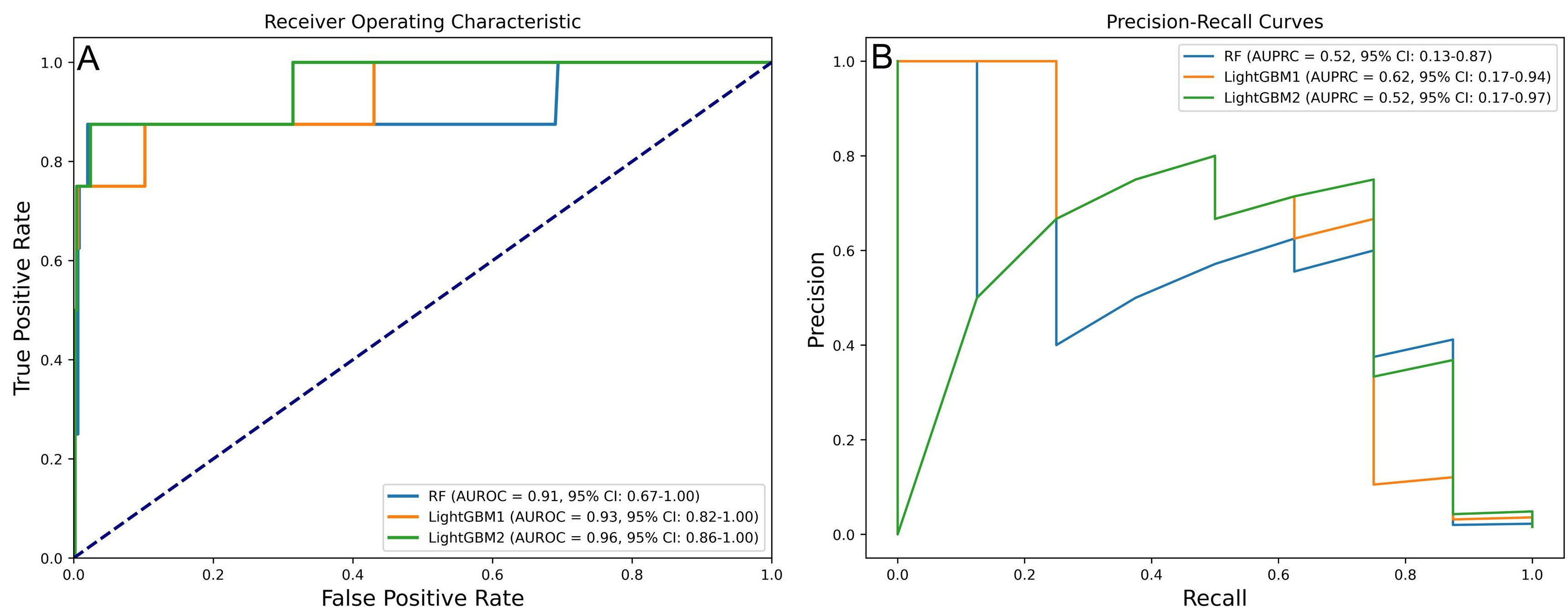Fig. 4.

Performance of three prospective models in predicting IHM post-PCI in AMI patients. (A) AUROC values of prospective models. (B) AUPRC values of prospective models.

To compare model performance, DeLong and bootstrap tests were applied to the AUROC and AUPRC values (Fig. 5). Although LightGBM1 outperformed the other models on both metrics, the differences were not statistically significant (p $>$ 0.05).

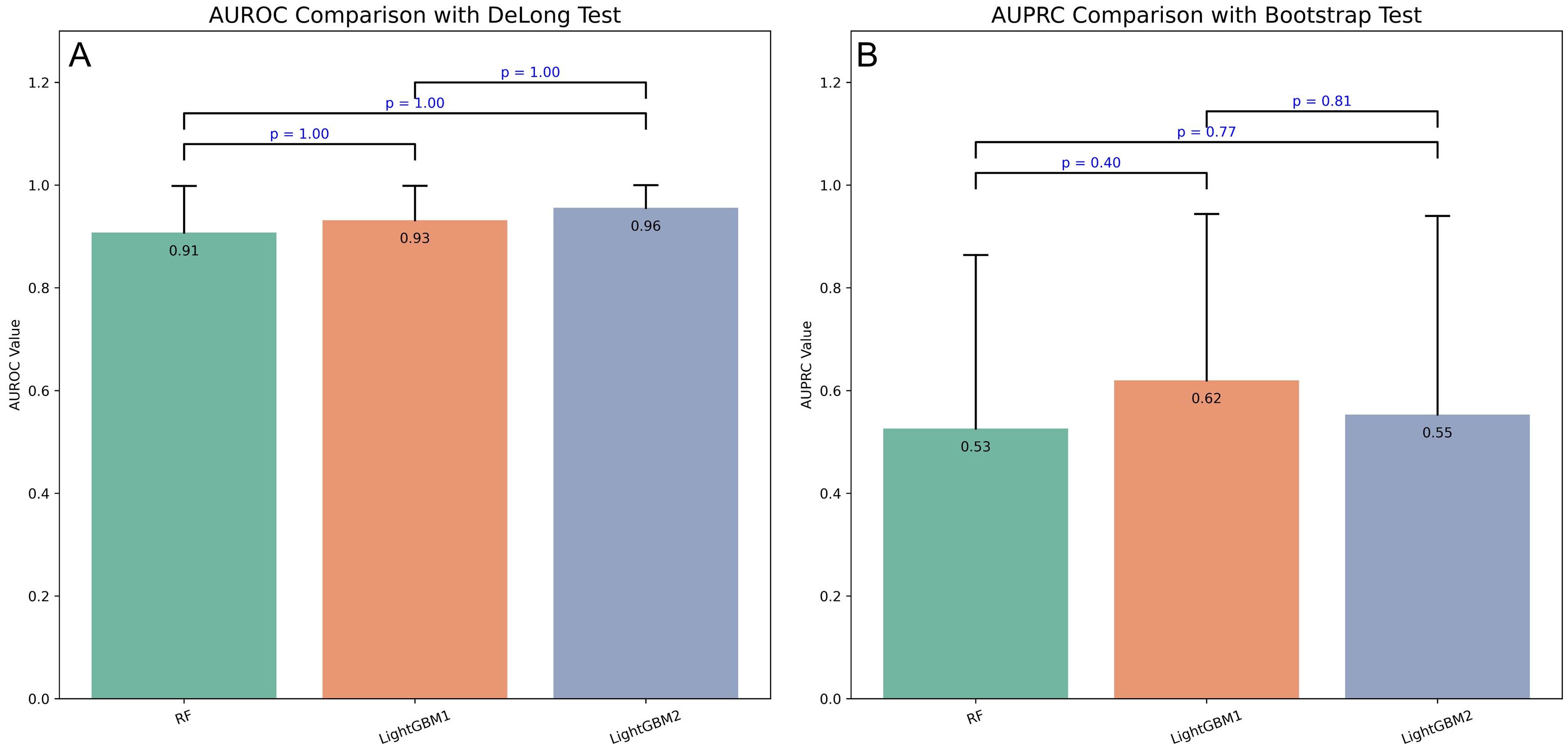Fig. 5.

Performance comparison of three prospective models using DeLong and bootstrap tests. (A) DeLong test comparing AUROC values across three prospective models. (B) Bootstrap test comparing AUPRC values across three prospective models.

Violin plots were employed to visualize the probability density distributions of AUROC and AUPRC (Fig. 6). The LightGBM1 model exhibited a more concentrated AUROC distribution compared to LightGBM2 (Fig. 6A). Its AUPRC distribution was right-skewed, with a median around 0.7, indicating superior discriminative ability (Fig. 6B).

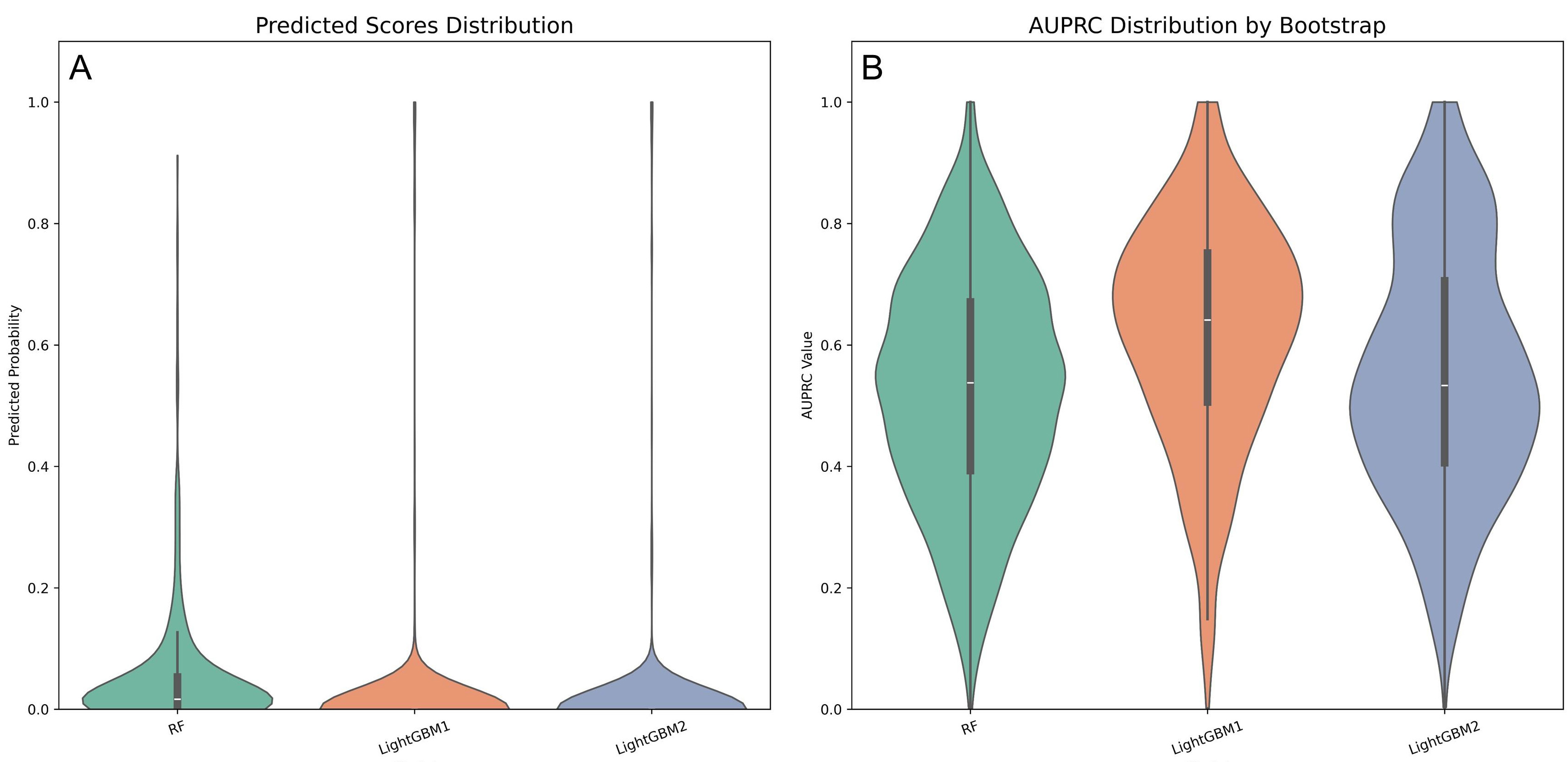Fig. 6.

Violin plots comparing performance metrics across three predictive models. (A) AUROC distribution of three prospective models. (B) AUPRC distribution of three prospective models.

The results of the first phase demonstrated no statistically significant differences in model performance across the various processing methods. While the combination of SMOTE, Boruta, and GSCV effectively reduced feature dimensionality, it may have compromised predictive efficacy. Consequently, the final comparison focused on SMOTE combined with GSCV and SMOTE combined with Boruta and GSCV to identify the optimal processing approach. In the second phase, LightGBM exhibited a slight performance advantage over RF, although this difference was not statistically significant, which led to the inclusion of both algorithms in the final evaluation. In the final phase, based on comparisons of AUPRC and violin plots, the configuration of SMOTE, Boruta, GSCV, and LightGBM was identified as the optimal model configuration.

The original dataset exhibited a significant class imbalance, which limited the effectiveness of various analytical algorithms. To facilitate robust model development, the class distribution was initially adjusted using the SMOTE, resulting in an increase in the number of deceased cases from 24 to 1159 (see Fig. 7).

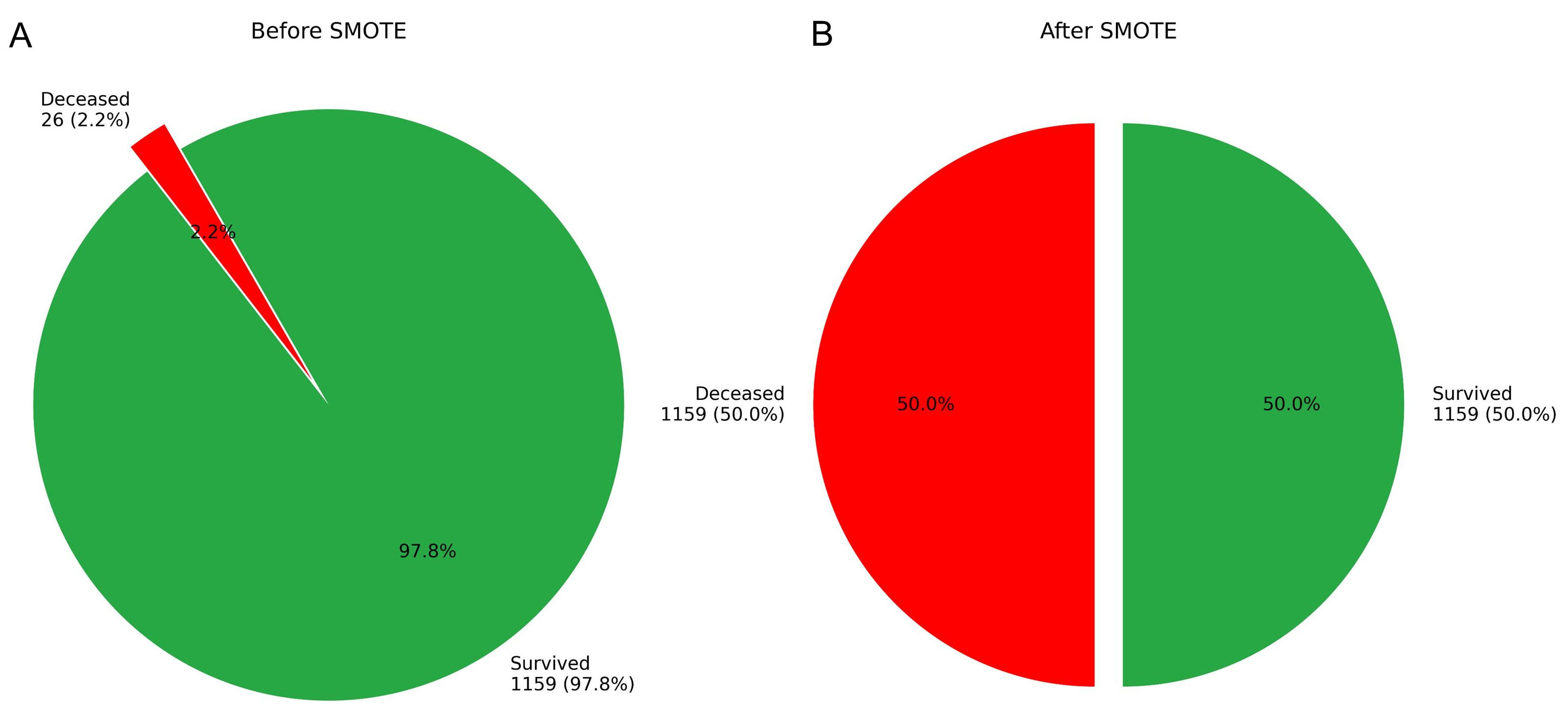Fig. 7.

Case distribution in the training cohort before and after SMOTE augmentation. (A) Original distribution. (B) Post-SMOTE distribution.

To reduce model complexity and mitigate the risk of overfitting, feature selection was conducted utilizing the Boruta algorithm, which decreased the number of predictors from 39 to 32.

The optimized LightGBM model was configured with the following parameters: min_samples_split = 5 (the minimum number of samples required to split a node), n_estimators = 200 (the number of boosting iterations), and random_state = 3331 (to ensure reproducibility). These hyperparameters were selected through grid search to achieve a balance between model performance and computational efficiency.

To enhance clinical interpretability and address concerns regarding the explainability of ML models, SHAP was employed to elucidate the final model’s output by quantifying the contribution of each feature to individual predictions. SHAP summary plots illustrate feature importance in descending order based on mean SHAP values (Fig. 8). Each point represents an individual sample, with rows corresponding to specific features. The horizontal axis denotes SHAP values, while the color gradient (red indicating high values and blue indicating low values) reflects the original value of the feature.

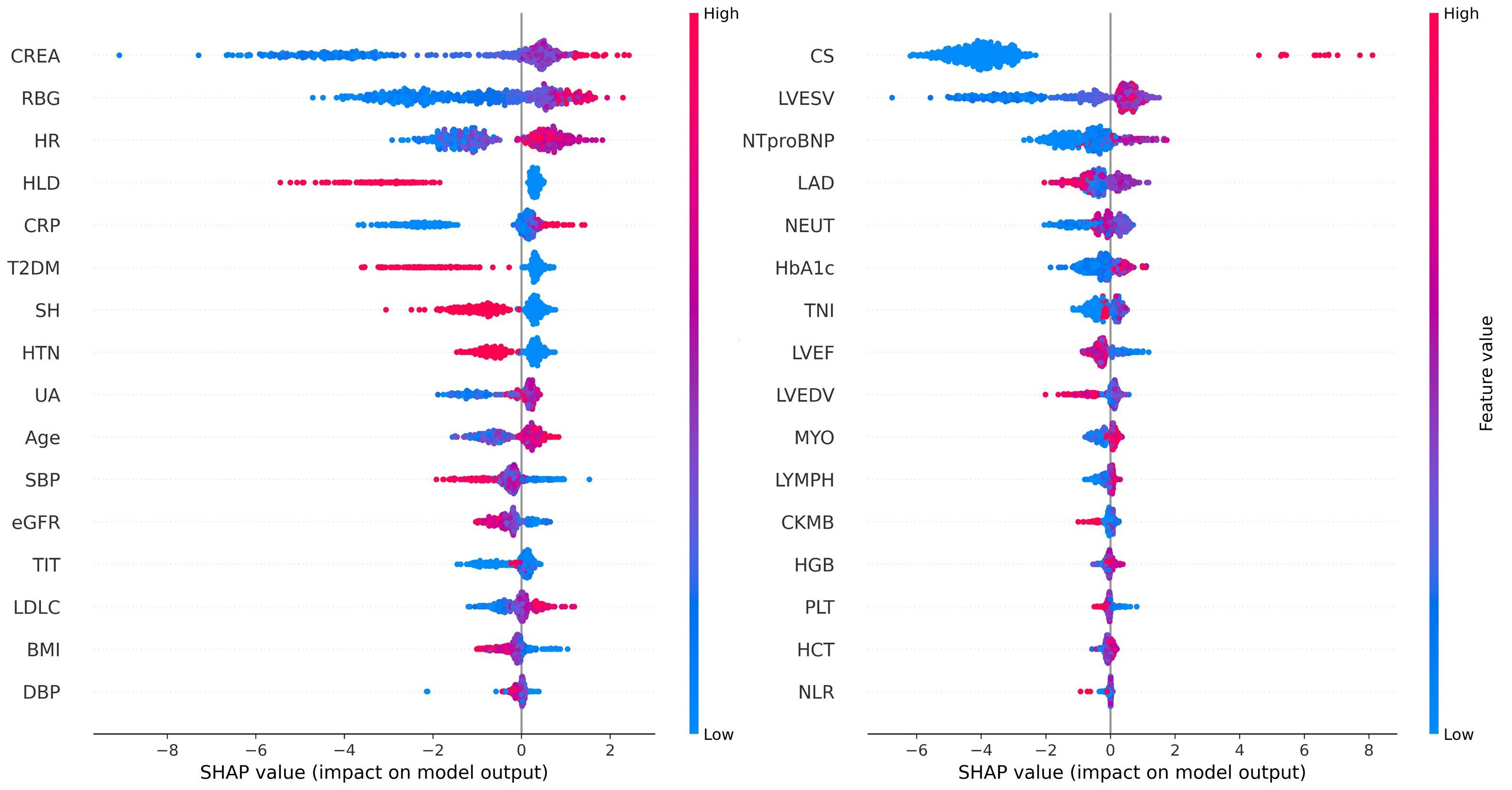Fig. 8.

SHAP summary plot for the LightGBM model predicting IHM in AMI patients post-PCI. The plot shows each feature’s contribution to the model’s predictions.

The feature importance in the LightGBM model is visualized using a radar plot (Fig. 9A) and a SHAP summary bar plot (Fig. 9B). Both visualizations highlight the top 13 predictors of IHM, ranked by their relative contributions. RBG was identified as the most influential variable, followed by CREA and CS.

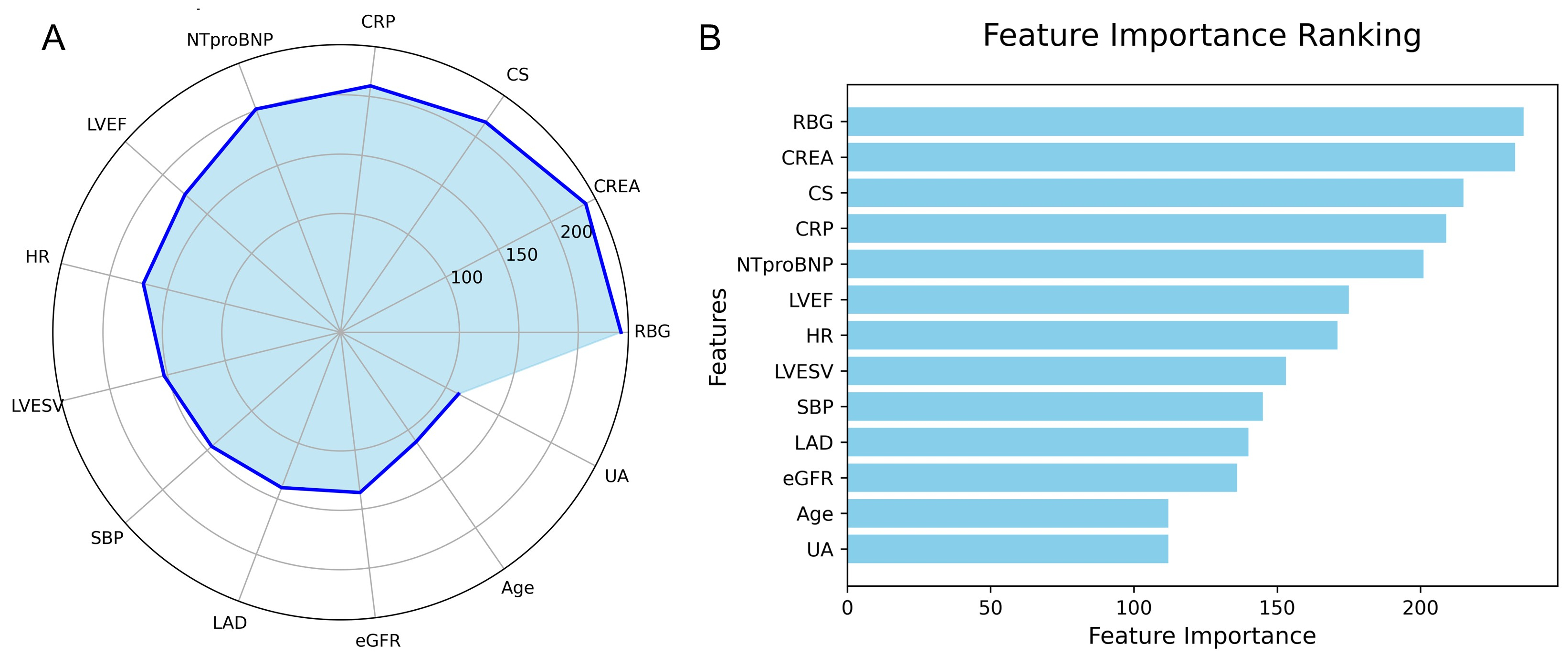Fig. 9.

Feature importance in the LightGBM model predicting IHM in AMI patients post-PCI. (A) Radar plot of feature importance. (B) SHAP bar plot showing individual feature contributions.

To enhance the clinical applicability of the model, the final predictive model has been deployed as a web-based application (Fig. 10). Clinicians are able to input values for the 32 required features, and the application automatically estimates the individual risk of IHM for patients with AMI. Additionally, it generates a personalized SHAP force plot that visually highlights the factors influencing each prediction. In these plots, the blue features on the right indicate variables associated with improved survival, while the red features on the left represent factors that contribute to an increased risk of mortality.

Fig. 10.

Clinical application of the LightGBM model for IHM prediction in AMI patients post-PCI. The application uses 32 input features to predict IHM probability (e.g., 37.1%). The accompanying SHAP force plot visualizes individual feature contributions: blue bars (right) push the prediction toward mortality, while red bars (left) favor survival.