


 , Yuequan Shi 1,†, Wenting Cao 1, Jingde Hong 2, Ming Li 2, Yuhang Xie 2, Zeng Lin 2, Yongping Lin 2,*
1 Department of Radiology, Fujian Maternity and Child Health Hospital & Fujian Key Laboratory of Women and Children’s Critical Diseases Research, 350001 Fuzhou, Fujian, China
2 School of Optoelectronic and Communication Engineering, Xiamen University of Technology, 361024 Xiamen, Fujian, China
†These authors contributed equally.
Abstract
Early diagnosis and accurate staging of endometrial cancer (EC) are crucial for effective treatment planning. Distinguishing stage IA from stage IB EC is challenging due to large variations in tumor and uterine morphology, as well as the limited availability of annotated magnetic resonance imaging (MRI) data for training robust models.
A genetic programming (GP)-based framework was developed for the classification of FIGO stage IA and IB EC using a small number of MRI images. The framework consists of three main components: (1) automatic detection of regions of interest (ROI) on MRI images, (2) GP-based feature extraction and construction, and (3) EC stage classification. A fast single-shot detector (SSD) was employed to automatically localize the uterus as the ROI. The detected ROI images were cropped and resized to construct training and test datasets. Four GP-based methods with different structures and primitives were employed for feature extraction and construction: GP with convolutional operators (COGP), GP with image descriptors (IDGP), GP with flexible program structures and image-related operators (FlexGP), and GP with automatic simultaneous learning of features and evolutionary ensembles (FELGP). The best-performing GP individuals were used to generate discriminative features, which were subsequently used to train classifiers for stage IA and IB EC.
Experimental results from three MRI datasets revealed that GP-based methods achieved competitive performance relative to both neural and traditional non-neural machine learning approaches. The proposed methods achieved classification accuracies of up to 0.92 on cropped axial diffusion-weighted imaging (DWI), 0.87 on cropped axial T2-weighted imaging (T2WI), and 0.83 on cropped sagittal T2WI images of EC patients.
GP-based methods effectively classify FIGO stage IA and IB endometrial cancer using limited MRI data. By automatically extracting discriminative and interpretable features from ROI within lesions, the proposed framework provides a reliable and transparent solution for EC staging, highlighting the potential of GP in medical image analysis and clinical decision support.
Keywords
- endometrial neoplasms
- genetic programming
- image analysis
- magnetic resonance imaging
Cancer of the corpus uteri, referred to as endometrial cancer (EC), arises from
the epithelial lining of the uterine cavity. The first local extension of EC
involves the myometrium [1]. The incidence of EC continues to increase globally
and is estimated to reach more than 400,000 cases annually [2]. Furthermore, the
incidence of early-onset EC (age at diagnosis
Magnetic resonance imaging (MRI) has significant value in assessing the extent of myometrial and cervical invasion, the extent of extra-uterine involvement, lymph node metastasis, and tumor size [11]. Due to the specialized nature and complexity of medical images, experienced clinicians are usually tasked with reviewing the patient’s MRI images, deciding the correct tumor stage, and recommending appropriate treatment strategies [12]. However, the ability to make a correct assessment based on pre-operative MRI images is primarily dependent on individual expertise and experience, which can often vary from one person to another [13].
Computer-aided diagnostic (CAD) methods based on artificial intelligence (AI) are now used to assist radiologists in analyzing MRI images of EC patients. To date, most studies on the use of MRI for EC are based on the machine learning (ML) method [14, 15, 16]. Many radiomics features for these ML-based classification models still require manual labeling of MRI images and a high level of domain knowledge and expert experience to extract representative features. Dong et al. [17] reported that the diagnostic accuracy of an AI classification model based on deep learning (DL) for T1-weighted images (T1WI) and T2-weighted images (T2WI) was 79.2% and 70.8%, respectively. Chen et al. [18] developed a classification model that combines Yolov3 with a convolutional neural network (CNN) to dichotomize MRI images of EC patients. This model achieved a sensitivity of 0.67, specificity of 0.88, and accuracy of 0.85. However, the performance of these classification methods is not satisfactory. Furthermore, although DL-based EC classification methods avoid the need for rich domain knowledge, they are less interpretative due to the “black-box” nature of DL models, often requiring large numbers of training images/samples. Obtaining a large number of training images is challenging due to hospital policies regarding patient privacy and discrepancies in MRI images across different institutions.
To overcome the above limitations, a genetic programming (GP) algorithm was developed that evolves solutions of different lengths based on a tree structure [19]. The evolutionary process for GP does not require special knowledge. GP programs/solutions can usually be translated into symbols because the presentation of programs is often a tree consisting of pre-defined functions. With this tree structure, GP can represent higher-level structures, giving it a unique advantage in solving complex problems. Solutions generated by GP are potentially highly interpretable [20]. GP has been applied to many fields, including fault diagnosis [21], edge detection [22], and action recognition [23]. GP has also shown strong potential for image classification, demonstrating excellent performance in the classification of low-quality images, as well as few-shot images [24, 25]. Nevertheless, relatively few studies to date have applied GP to the classification of medical images [26, 27], and none have applied this technique to automatically classify early EC patients into stage IA and IB.
This study has two overall aims. The first is to apply existing GP-based classifiers to distinguish stage IA and stage IB EC on MRI images. The second is to compare the classification performance of GP to that of neural or non-neural ML-based classification models. The main contributions of this work can be summarized as follows:
(1) The GP approach was applied to the classification of a small number of stage IA and IB EC samples, achieving good results.
(2) The GP approach uses object detection to reduce redundant information in MRI images of the uterus. Combined with DL, this reduces computational resources, allowing the GP model to achieve more accurate classification while making the medical image diagnosis process more interpretable.
GP is an evolutionary computation technique that uses the principles of Darwinian evolution to automatically discover computer programs. In this population-based algorithm, each individual in the population (model or tree) represents a candidate solution to a problem [28]. GP utilizes selection, elitism, crossover, and mutation in evolution to renew populations. A flowchart of the GP algorithm is shown in Fig. 1. Many of these issues have been addressed incrementally, leading to more widespread application of GP in various domains.
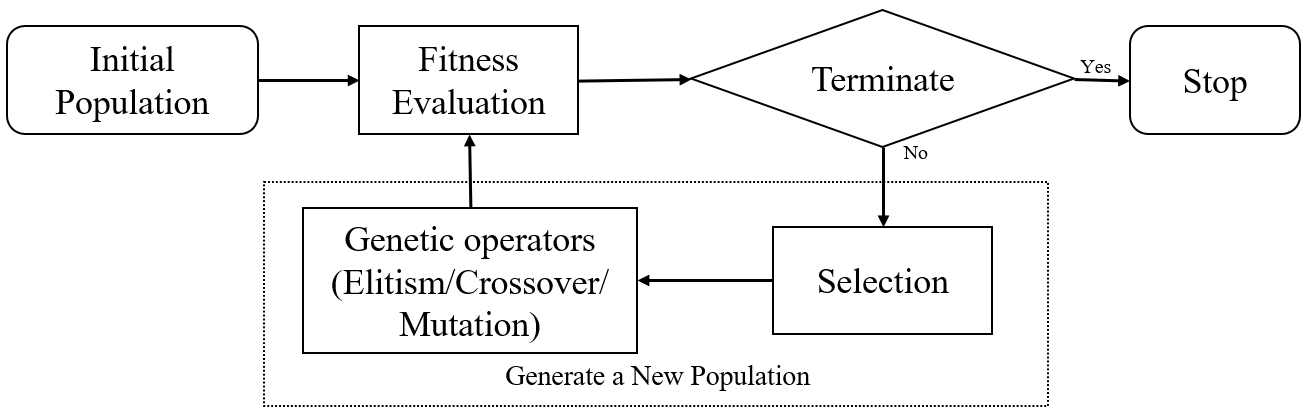 Fig. 1.
Flowchart of the GP algorithm. The algorithm starts with an initial population, followed by fitness evaluation and selection. Genetic operators, including elitism, crossover, and mutation, are applied to generate new populations iteratively until a termination condition is met. GP, genetic programming.
Object detection is a computer technology related to computer vision and image processing that involves the detection of certain types of semantic objects (e.g., humans, buildings, or cars) in digital images and videos [29]. Most of the current state of-the-art object detectors are based on DL networks, which mainly use the backbone network for feature extraction of the input image or video, and the detection network for classification and localization. Mainstream object detectors are usually divided into two-stage detection (represented by Faster-RCNN [30]), one-stage detection (represented by YOLOv3 [31]), and a fast single-shot object detector (SSD) [32]. The one-stage detector has a high inference speed, while the two-stage detector has high object recognition accuracy. These object detectors have found a wide range of applications in medical imaging, including COVID-19 detection on X-ray images [33], lung nodule detection on computed tomographic (CT) images [34], and the detection of EC lesions on MRI images [18].
The fundamental principle of the proposed stage IA and IB EC classification method is to crop out the ROI in MRI images through the object detection model, thereby reducing the computational cost of GP and interference from irrelevant information. The flowchart for the proposed GP-based classification method for distinguishing FIGO stage IA and IB EC involves three steps, as shown in Fig. 2.
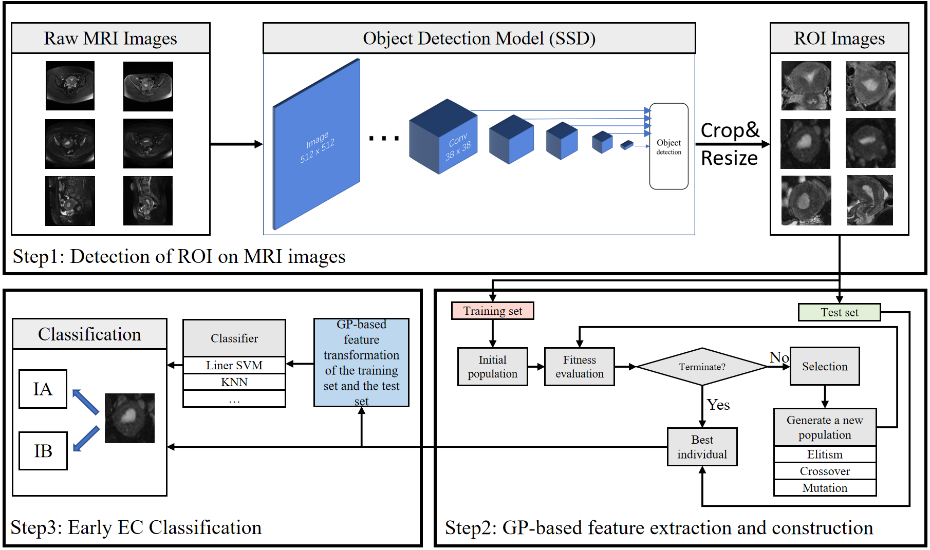 Fig. 2.
Flowchart of the proposed GP-based framework for classifying stage IA and IB endometrial cancer (EC). This consists of three stages: (1) ROI detection on MRI images using an SSD-based object detection model, followed by cropping and resizing of the detected regions; (2) GP-based feature extraction and construction from the ROI images; and (3) classification of stage IA and IB EC using the GP-extracted features with conventional classifiers. Arrows indicate the data flow between different stages. Abbreviations: MRI, magnetic resonance imaging; ROI, region of interest; GP, genetic programming; SSD, single shot multibox detector; EC, endometrial cancer.
Step 1: Detection of the ROI in MRI images. The ROI in MRI images is detected
using a DL-based object detection network, then cropped out based on the
detection of the resulting bounding box. The network employs an SSD model with
pretrained weights from the Visual Object Classes (VOC) 2007 dataset [35], as
detailed in Section 3.1.2. Through pre-training, it can learn the commonality of
images, transfer the commonality to the task-specific model, and then fine-tune
the model using a small number of samples. The training process consisted of 100
epochs, during which the first 21 layers of the pre-trained model had their
parameters frozen for the first 50 epochs. The entire network’s parameters were
then updated in the remaining 50 epochs. The technique of freezing layer
parameters was employed to control weight updates during training, thus
preventing over-adjustment and improving model performance and robustness in
fine-tuning pre-trained models. The input images for training the SSD are the raw
images and coordinates of the bounding boxes, as depicted by the radiologist. The
ROI images are cropped and resized to 150
Step 2: GP-based feature extraction and reconstruction. Features are extracted and constructed from MRI images using GP. In GP, populations are evolved using fitness assessment and genetic operators. Each individual in the population represents a solution that allows a flexible number of features to be extracted from the MRI images. The fitness assessment guides the evolution of the GP. When the number of generations reaches a termination condition, the whole evolutionary process stops, and the best individual (i.e., the one with the highest fitness) is returned. The best individuals evolved by the GP are used to classify the test sets.
Step 3: Stage IA and IB EC classification. FELGP is an ensemble learning approach, with internal training of classifiers and a voting mechanism that allows direct predictions to be made on class labels. The other three GP methods require normalization of the extracted and constructed features. The normalized features of the training set and the corresponding class labels are fed into a classification algorithm (e.g., linear Support Vector Machine [SVM], K Nearest Neighbors [KNN]). Finally, the images in the test set are converted into feature vectors by the GP program, which are then used to train the classifier.
SSD is an object detection method using deep NN [32]. This study used SSD for ROI detection on raw MRI images. SSD first extracts convolutional features in images using the VGG network. These are subsequently used to generate feature maps at different scales. The feature maps contain information about objects of different sizes and proportions, enabling SSD to detect objects of different sizes. The bounding box output space at each position on the feature map is then discretized into a set of default boxes with different aspect ratios and proportions. Each default box predicts the confidence of its internal object class and the offset relative to the ground truth box. The ratio of positive and negative samples is controlled by two methods: non-maximum suppression (NMS) and hard negative mining. NMS is a technique used to remove redundant bounding box predictions. It involves sorting bounding boxes by confidence scores, selecting the one with the highest score, and then eliminating others with significant overlap. This process is repeated until all boxes are processed, resulting in improved accuracy by retaining only the most accurate and non-overlapping predictions. Hard negative mining is another training strategy in object detection algorithms that focuses on selecting challenging negative samples. It involves identifying misclassified or high-confidence negative samples and incorporating them into the training set to improve the model’s ability to distinguish objects from background regions. This iterative process enhances the model’s performance in complex scenarios. The SSD approach encapsulates all necessary computations within a single network, making it straightforward to compute and seamlessly integrate stage IA and IB EC classification as a detection component. A previous study found that the SSD model easily covers the uterus region [36]. Moreover, with the same training dataset, the SSD model has fewer parameters than other detection models, reducing the computational resources.
In this study, four existing GP-based classifiers were chosen based on the following criteria: (1) whether they can be applied to image classification tasks; (2) whether they can automatically learn effective features from images; and (3) whether they require a large number of training examples. Accordingly, four different STGP representations with different functionalities were adapted to stage the MRI images of EC. The four GP methods [20] based on STGP were: (1) GP-based method with convolution operators (COGP)—applied to feature learning in images for classification; (2) GP-based method with image descriptors (IDGP)—applied to learning global or local features in images for classification; (3) GP-based method with a flexible program structure and image-related operators (FlexGP)—applied to feature learning in image classification; and (4) GP-based method with feature ensemble learning (FELGP)—applied to automatically and simultaneously learn features and evolve ensembles in images for classification.
To validate the effectiveness of the framework, each GP-based classifier (COGP, IDGP, FlexGP, and FELGP) was separately employed in the framework for feature extraction to classify MRI images of EC patients. The structure of these programs is shown in Fig. 3. The individual characterization methods of the four GP methods are different from each other. The program structure of COGP is inspired by CNNs [20]. It has convolution and pooling operations, which are used to extract features in GP programs. In addition, a distinctive feature of the COGP program structure is its combination of fixed and flexible layers. The fixed layers of this program structure serve to facilitate feature transformation and dimensionality reduction, while the flexible layers enable the evolution of trees of varying sizes based on the complexity of the task. IDGP has a novel program structure that automatically selects and combines existing image descriptors, such as Local Binary Pattern (LBP), Histogram of Oriented Gradients (HOG), and Scale-Invariant Feature Transform (SIFT). This occurs in a flexible manner to extract rich and discriminative global and/or local features for different image classification tasks. The program structure of FlexGP combines two different types of features: those extracted through filtering/pooling, and those extracted through traditional feature extraction methods. This flexible structure enables FlexGP to generate a diverse range of feature types and quantities. The method evolved by FlexGP produces variable-length solutions that can extract an array of features from raw images. Lastly, the FELGP approach extracts features and integrates the classification algorithms automatically. It is worth noting that while all methods utilize MRI images as input, their outputs differ. The first three methods (COGP, IDGP, and FlexGP) generate learned features from the image, which are then used to obtain class labels through various classifiers. In contrast, FELGP functions as an ensemble learning approach, with internal classifier training and a voting mechanism that enables direct predictions on class labels. The implementation source codes for the above four GP methods are available at https://github.com/XL9984/GP-ECMRI.
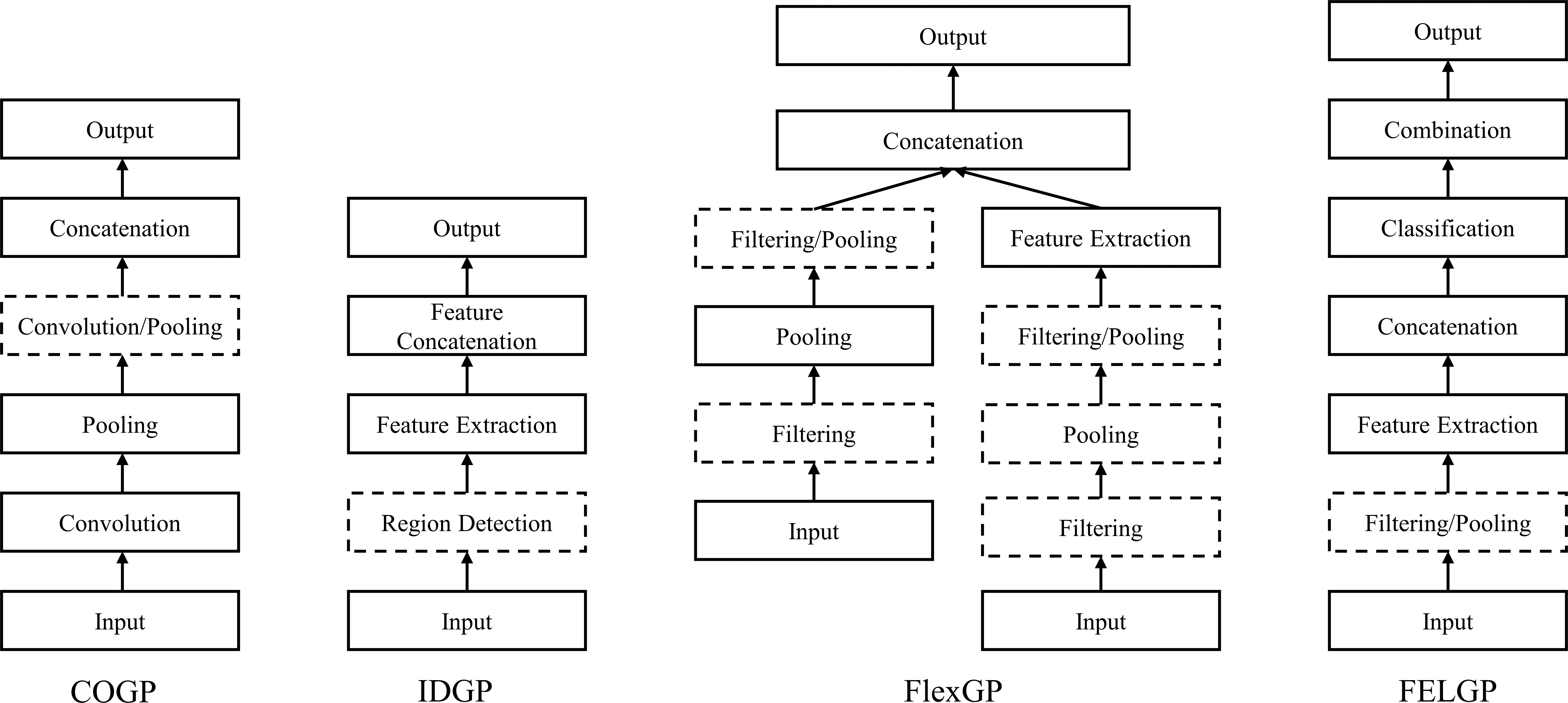 Fig. 3.
The structures of four GP-based methods. COGP employs convolution operators for image feature learning. IDGP utilizes image descriptors to extract global or local features. FlexGP adopts a flexible program structure with image-related operators. FELGP integrates feature learning with ensemble evolution for image classification. Abbreviations: GP, genetic programming; COGP, convolution-operator-based GP; IDGP, image-descriptor-based GP; FlexGP, flexible-structure GP; FELGP, feature-ensemble-learning GP.
In this subsection, the proposed approach for classifying early EC patients was verified on three MRI datasets: axial diffusion-weighted imaging [DWI], axial T2WI, and sagittal T2WI images. The data and baseline classification methods used for comparison, experiments, and parameter settings are presented in this subsection.
The Institutional Review Board (IRB) of Fujian Maternity and Child Health Hospital (FMCHH) in China approved this retrospective study (No. 2025KY166). The requirement for informed consent was waived. A total of 207 patients clinically suspected of EC underwent 1.5T MRI before undergoing surgery in Fujian Maternal and Child Health Hospital from January 1, 2018, to December 31, 2020. Because this study was focused on MRI-based classification of early-stage EC, patients with stage II, III, and IV disease were excluded. The classification task was restricted to FIGO stage IA and IB, which are defined by the depth of myometrial invasion and can be assessed using preoperative MRI [37]. The additional inclusion criteria were as follows: (1) a clear MRI slice image of the uterus; (2) T2WI images had corresponding DWI images; and (3) the existence of a final pathological diagnosis result. The final number of enrolled EC patients meeting the criterion was 100, with an average age of 55.7 years. These comprised 43 patients with stage IA EC and 57 patients with stage IB EC. The experimental data consists of three modalities, as shown in Fig. 4. Detailed clinicopathological characteristics of the enrolled patients are summarized in Table 1.
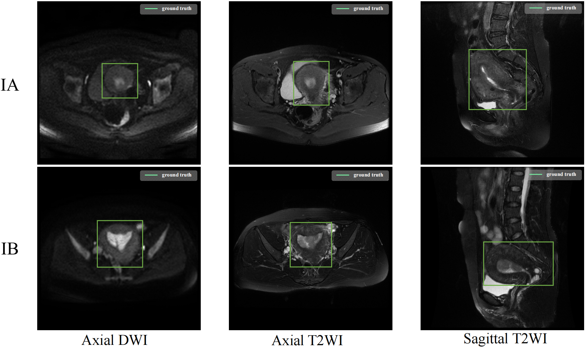 Fig. 4.
The labelled ROI in MRI images. The figure shows representative ROI annotations for the three MRI modalities used in this study, including axial diffusion-weighted imaging (DWI), axial T2-weighted imaging (T2WI), and sagittal T2WI.
| Parameter | Stage IA (n = 43) | Stage IB (n = 57) | Total (n = 100) | p-value | |
| Average age (years) | 51.4 |
58.9 |
55.7 |
||
| Endometrioid type# | 0.239 | ||||
| Grade 1 | 27 | 28 | 55 | ||
| Grade 2 | 15 | 24 | 39 | ||
| Grade 3 | 1 | 5 | 6 | ||
| Maximum diameter (cm) | |||||
| 32 | 19 | 51 | |||
| 11 | 38 | 49 | |||
| Myometrial invasion | |||||
| 43 | 3 | 46 | |||
| 0 | 54 | 54 | |||
| Mixed carcinoma* | 0.245 | ||||
| No | 29 | 32 | 61 | ||
| Yes | 14 | 25 | 39 | ||
# Histological grading of endometrioid carcinoma. According to the solid
range of tumors, the classification criteria are as follows: Grade 1: solid
growth area accounts for
* Indicates the presence of other tumors, such as clear cell carcinoma, uterine fibroids, etc.
Seventy cases (30 stage IA and 40 stage IB) were randomly selected as the
training set, and 30 cases (13 stage IA and 17 stage IB) as the test set. For
each case, appropriate MRI images were selected by two experienced radiologists
with over 20 years of clinical experience, resulting in a total of 300 images.
These were divided into three datasets: 100 axial DWI images, 100 axial T2WI
images, and 100 sagittal T2WI images. The original MRI image size was 512
To demonstrate the effectiveness of the GP-based methods, two different types of methods were used for comparison. The first method is based on four classification algorithms that are classical ML methods: support vector machine (SVM), K-Nearest Neighbours (KNN), linear regression (LR), and multilayer perceptron (MLP). To ensure a fair comparison of classification accuracy, these algorithms take the raw images (standardized input) for each method, rather than relying on extracted features. By doing so, the performance of each method can be evaluated on the same input data, avoiding potential bias that may arise from using different feature extraction methods. The comparison aims to determine whether the features extracted and constructed by GP are more effective for EC classification. The second method involves four classification algorithms based on DL methods: ResNet50, VGG16, InceptionV3, Xception, EfficientNetV2-small, and Vision Transformer-small (ViT). These classification algorithms also use the raw images as inputs, whereas the internal network structure learns certain image features before classifying them. The comparison determines whether the GP-based approach is more effective than the DL-based approach when using a small amount of data.
The functions of FELGP are listed in Table 2. The function set incorporated in this study comprises a diverse range of functions, each designed to serve a unique purpose. Table 3 lists the terminal set of FELGP.
| Function | Input/output | Description |
| Gau | Img/Img | Gaussian filtering |
| LoG | Img/Img | Laplacian filtering |
| W-Sub | Img,Float/Img | Subtract two weighted images |
| HOG | Img/Vector | HOG descriptor |
| SIFT | Img/Vector | SIFT descriptor |
| uLBP | Img/Vector | 59 uniform LBP descriptor |
| FeaCon | Img/Vector | Convert images to a vector by concatenating each row |
| ERF | Vector/Vector | Perform ERF (Extreme Random Forests) method to get label |
| SVM | Vector/Vector | Perform SVM method to get label |
| Comb | Vector/Vector | Concatenate two vectors to a vector |
| Terminal | Data type | Description |
| X train | Arrays1 | All the training images |
| Y train | Arrays2 | The labels of the training images |
| Integer | The standard deviation of the Gaussian filter | |
| Integer | The orders of the Gaussian derivatives | |
| Float | The orientation of the Gabor function | |
| f | Float | The frequency of the Gabor function |
| n1, n2 | Float | The parameters of the W-Add and W-Sub |
| k1, k2 | Integer | The kernel size for MaxP |
| C | Integer | The penalty term/parameter in SVM is 10C |
| NT | Integer | The number of trees in ERF |
| MD | Integer | The maximum depth of the decision tree |
To keep the comparison fair, the same parameters are used for different GP methods. The number of GP individuals in a GP population is set to 100 to save computational time, since the processing of images at the pixel level is a time-consuming task [39]. The initial GP population is generated using the ramped half-and-half method, which is the commonly used population initialization method in image processing applications [40]. This method enhances program diversity by producing an initial tree with variable length, facilitating the combination and integration of program fragments to create more complex and hopefully fitter programs [41]. The tournament selection strategy is employed to maintain population diversity, with a tournament size set to 7. The advantage of this method is that it helps to maintain constant selection pressure. Even programs with average fitness have the opportunity to reproduce a child in the coming generation. The mutation, crossover, and elitism rates are 0.19, 0.80, and 0.01, respectively. As a result, the optimal parameter settings for the four GP methods are obtained in the commonly used settings in the community of GP [20].
The flowchart for ROI detection is shown in Fig. 5. The confidence was set to 0.75 to display more accurate results, where confidence refers to the ratio of the intersection to the union between the detection result and the ground truth. In the test set, the model with pre-training weights from the VOC dataset achieved an average precision (AP) of 95.81% with all three kinds of MRI images. The model with pre-training weights from the Common Objects in Context (COCO) dataset achieved an AP of 87.46% on the same set of MRI images. However, the detection model without pre-training had an AP of only 77.19%. The precision-recall (PR) curves for the three models of ROI detection are shown in Fig. 6. The horizontal axis of each subplot represents the recall, while the vertical axis represents precision. The PR curves indicate the detection model with pre-training performed exceptionally well and could accurately localize the ROI (i.e., the uterine region). This model was used in the first step of Fig. 2 to process all MRI images and obtain the corresponding ROI images.
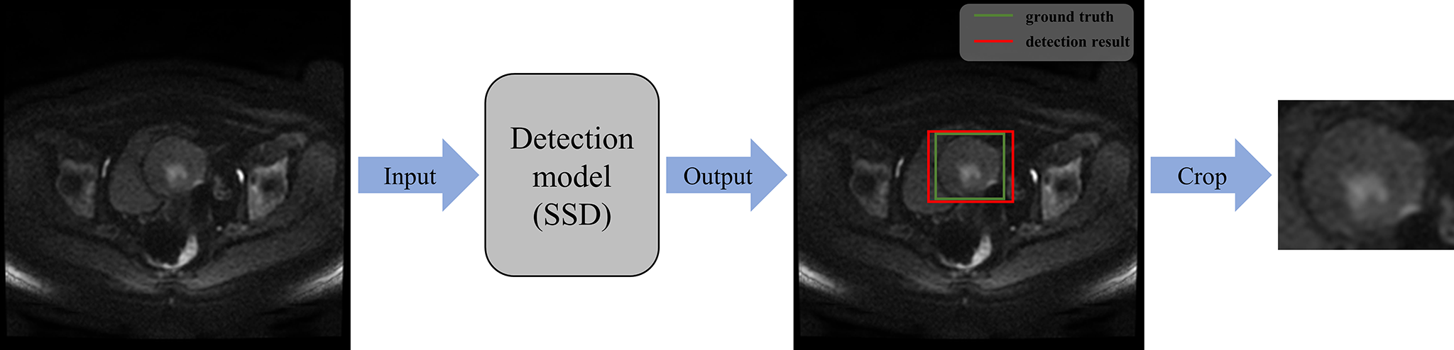 Fig. 5.
Flowchart for ROI detection on MRI images. The SSD-based detection model localizes the uterine region on MRI images, followed by cropping and resizing to obtain the ROI images.
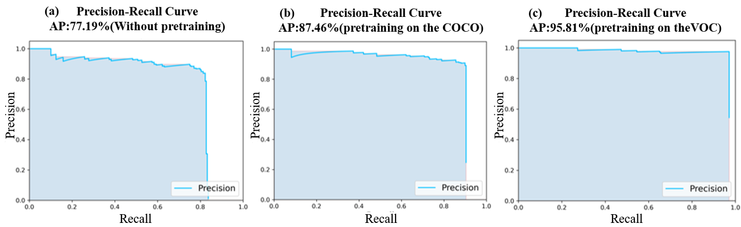 Fig. 6.
PR curve for ROI detection on MRI images. (a) Detection model trained without pre-training; (b) detection model pre-trained on the Common Objects in Context (COCO) dataset; and (c) detection model pre-trained on the Visual Object Classes (VOC) dataset.
The results of the GP-based methods and of the baseline methods for stage IA and IB EC classification on the three types of MRI images are shown in Table 4. The best classification results for each dataset are highlighted in bold. In addition, the accuracy of the classification of the boxed ROI images was tested against that of the raw images. The Wilcoxon Rank Sum Test was utilized to analyze the experimental results and assess the impact of incorporating object detection on the classification accuracy. The resulting significant data was used to identify potential differences between the two groups of data (raw MRI images and ROI images). The Wilcoxon Rank Sum Test was conducted across three distinct methodologies, including ML-based methods, DL-based methods, and GP-based methods.
| Method | Axial DWI (Avg |
Axial T2WI (Avg |
Sagittal T2WI (Avg | ||||
| Raw | ROI | Raw | ROI | Raw | ROI | ||
| ML | SVM | 0.70 |
0.74 |
0.57 |
0.70 |
0.57 |
0.73 |
| KNN (K = 3) | 0.60 |
0.67 |
0.47 |
0.63 |
0.50 |
0.63 | |
| LR | 0.67 |
0.77 |
0.60 |
0.77 |
0.54 |
0.57 | |
| MLP | 0.50 |
0.73 |
0.57 |
0.67 |
0.47 |
0.60 | |
| p-value | |||||||
| DL | Resnet50 | 0.53 |
0.51 |
0.54 |
0.49 |
0.53 |
0.61 |
| Vgg16 | 0.48 |
0.57 |
0.49 |
0.60 |
0.49 |
0.51 | |
| InceptionV3 | 0.57 |
0.67 |
0.51 |
0.59 |
0.49 |
0.54 | |
| Xception | 0.53 |
0.47 |
0.51 |
0.52 |
0.52 |
0.61 | |
| EfficientNetV2-small | 0.60 |
0.67 |
0.55 |
0.55 |
0.50 |
0.58 | |
| ViT | 0.44 |
0.85 |
0.49 |
0.64 |
0.45 |
0.74 | |
| p-value | |||||||
| GP | COGP | 0.53 |
0.74 |
0.50 |
0.59 |
0.53 |
0.76 |
| IDGP | 0.52 |
0.77 |
0.45 |
0.63 |
0.43 |
0.83 | |
| FlexGP | 0.46 |
0.87 |
0.50 |
0.63 |
0.60 |
0.65 | |
| FELGP | 0.52 |
0.92 |
0.63 |
0.87 |
0.48 |
0.83 | |
| p-value | |||||||
Note: Raw: original MRI image; ROI: cropped image after detection by object detection model.
The first four rows of Table 4 show the classification results based on the ML classification algorithm. The classification accuracies were higher on ROI images than on raw MRI images. A significant difference was observed between the raw MRI images and ROI images on Axial T2WI and Sagittal T2WI images. The highest classification accuracy was 0.77 on ROI images of Axial DWI and Axial T2WI images using LR. These results indicate that cropped ROI images help to classify stage IA and IB EC better than raw MRI images. The raw images and ROI images on Axial DWI showed no significant difference, mainly because the DWI images highlight tumor lesions.
Rows 6 to 11 of Table 4 show the classification results based on the DL
classification algorithm. No significant improvement in classification accuracy
based on ROI images was observed compared to raw MRI images. Moreover, no
significant differences were observed between raw MRI images and ROI images on
Axial DWI and Axial T2WI images at the 0.05 significance level (all
p-values
Rows 11 to 14 of Table 4 show the classification results based on the GP
classification algorithms. The classification accuracies were significantly
higher on the ROI images than on the raw MRI images. A significant difference was
found between the raw MRI images and the ROI images (p
Columns 1, 3, and 5 of Table 4 show the classification results from the raw MRI images, while columns 2, 4, and 6 show the classification results from ROI images. None of the classification methods achieved a good result from the raw images, with accuracies of between 0.40 and 0.60. In contrast, the classification accuracies were higher with the ROI images. The FELGP-based classification method performed better on the ROI images than the ML- and DL-based classification algorithms. These results indicate that cropped ROI images improve the classification accuracy of all employed algorithms for the classification of stage IA and IB EC. In summary, GP-based algorithms are more effective than ML-based and DL-based classification algorithms.
Since the diagnosis of stage IA and IB EC is a dichotomous problem, a classifier should not be judged solely on its classification accuracy. To better illustrate that cropped ROI images help GP with feature extraction and construction, the receiver operating characteristic curves (ROC curves) and the area under the curve (AUC) of the four GP-based methods were compared to those of the raw MRI images and the ROI images (Fig. 7). The horizontal axis of each subplot represents the false positive rate (FPR), while the vertical axis represents the true positive rate (TPR). As shown in Fig. 7, the classification performance of the four GP-based classification methods on ROI images was significantly better than that of the raw MRI images. FlexGP and FELGP showed the best classification performances on ROI images of axial DWI images, with AUCs of 0.92 and 0.96, respectively. IDGP also demonstrated good classification performance on sagittal T2WI images, with an AUC of 0.92. In summary, the use of ROI images can help GP extract and construct valuable image features, thereby improving the accuracy and reliability of the classifier. Additionally, the classifier’s reliability is often more important in the diagnosis of medical images.
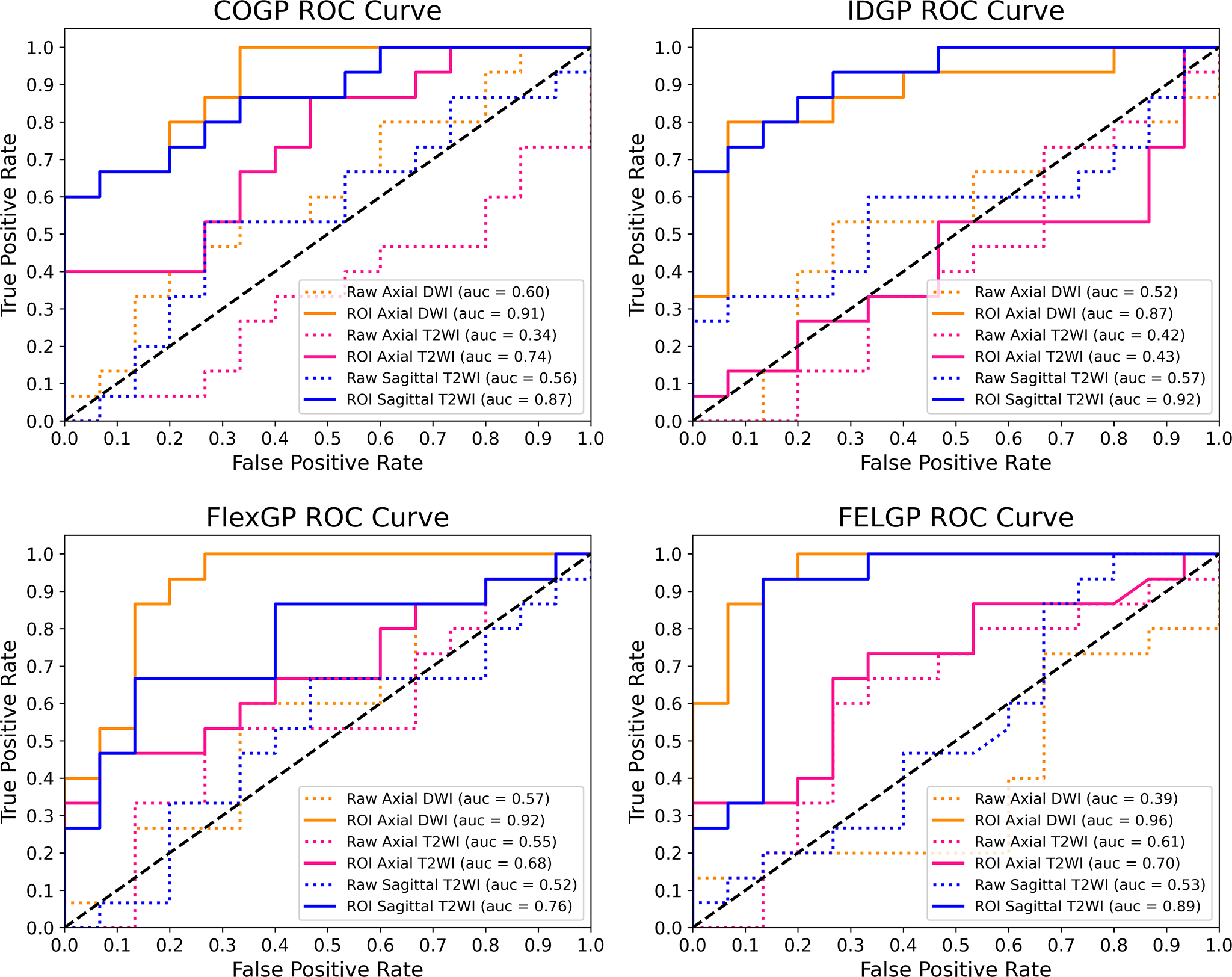 Fig. 7.
ROC Curves for the four GP-based methods. These compare the classification performance of COGP, IDGP, FlexGP, and FELGP using raw MRI images and the corresponding ROI images. The horizontal axis represents the false positive rate (FPR), and the vertical axis represents the true positive rate (TPR). Abbreviations: GP, genetic programming; ROI, region of interest.
As shown in Table 5, executing the process of evolutionary learning (step 2) is
time-consuming. The experiments based on DL methods were conducted on another
computer equipped with a high-performance Graphics Processing Unit (GPU). This
allows faster model training compared to other methods that run on a Central
Processing Unit (CPU), with a computation time on small datasets of
| Evolutionary learning time (hours) | ||||||
| Method | Axial DWI (Avg/Med) | Axial T2WI (Avg/Med) | Sagittal T2WI (Avg/Med) | |||
| Raw | ROI | Raw | ROI | Raw | ROI | |
| COGP | 12.87/12.17 | 1.93/0.88 | 11.29/13.11 | 0.22/0.27 | 5.59/4.82 | 1.76/2.10 |
| IDGP | 0.17/0.14 | 0.05/0.03 | 0.23/0.21 | 0.05/0.04 | 0.56/0.56 | 0.07/0.06 |
| FlexGP | 22.19/22.70 | 3.18/2.95 | 16.94/15.01 | 6.86/4.06 | 28.68/24.68 | 1.89/1.73 |
| FELGP | 237.03/217.75 | 31.27/19.83 | 224.28/190.98 | 30.20/30.14 | 127.56/119.59 | 25.75/23.26 |
| Evolutionary execution time (seconds) | ||||||
| COGP | 3.06/3.00 | 0.31/0.20 | 5.59/5.68 | 0.21/0.23 | 3.52/3.56 | 0.30/0.23 |
| IDGP | 0.04/0.03 | 0.01/0.02 | 0.01/0.02 | 0.00/0.00 | 0.02/0.03 | 0.02/0.01 |
| FlexGP | 6.24/6.28 | 1.33/1.09 | 9.44/9.64 | 6.33/6.40 | 12.89/12.80 | 0.75/0.66 |
| FELGP | 305.06/261.55 | 50.71/38.69 | 293.31/266.55 | 44.99/39.28 | 117.56/126.15 | 30.91/30.60 |
Table 5 shows the evolutionary learning time (in hours) and the execution times
(in seconds) of the GP-based methods. A significant difference was observed
between different GP methods for the same modality (p
Fig. 8 shows the best individual evolved by FELGP on the ROI image from axial DWI. Accuracies of 98.57% and 92.00% were achieved on the training and test sets, respectively. The relatively small gap between training and testing performance indicates that this representative FELGP model generalized well to unseen data, suggesting limited overfitting in this example despite being trained on a small dataset. This tree/program structure illustrates how valuable features are extracted from ROI images, and how effective classification of stage IA and IB EC is achieved. The GP method uses different features and functions to train the GP programs shown in Fig. 8. To illustrate the interpretability of the GP, the SVM classifier branch at the bottom of Fig. 8 is further visualized in Fig. 9. This shows how the GP extracts features, with two example images from stage IA and stage IB as inputs. As shown in Fig. 9, the image undergoes initial processing using various filtering and pooling functions to enhance the informative image characteristics. Edge filters (LoG1, LoG2, LaP, SobelX) are employed for extracting edges and textures, while blur/smoothing filters (Gau, Gabor) reduce image noise. The weight operator (W-sub) is mainly used to weight the image in order to highlight crucial information. Subsequently, the processed images undergo a feature extraction function (HOG, SIFT, uLBP) to obtain specific image features such as gradient direction, unique key points, and local texture patterns. These features are combined through the feature concatenation function to create high-level features suitable for classification. The high-level feature vectors and some image information are then fed into the classification algorithms, such as SVM and extreme random forests (ERF), as new features for training. Lastly, the final classification result output is obtained using an ensemble of the three classifiers. Overall, this structure allows different numbers and types of features to be extracted from the image, and the corresponding filtering and pooling operations to be performed under each branch to construct the high-level features. The ensemble learning approach enhances the robustness of this classification algorithm and improves its performance.
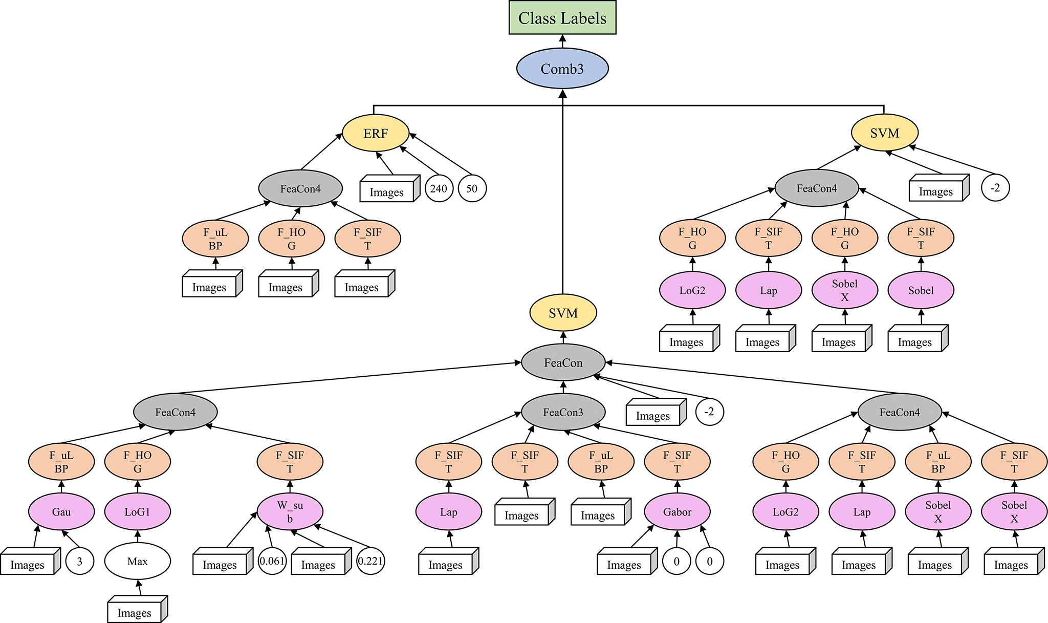 Fig. 8.
Example solution found by FELGP on axial DWI ROI images. This shows the best individual evolved by FELGP on the ROI image from axial DWI. The tree/program structure illustrates how image features are extracted using edge filters, blur/smoothing filters, and weight operators for the classification of stage IA and IB EC. Abbreviations: FELGP, feature-ensemble-learning genetic programming; DWI, diffusion-weighted imaging; ROI, region of interest; EC, endometrial cancer.
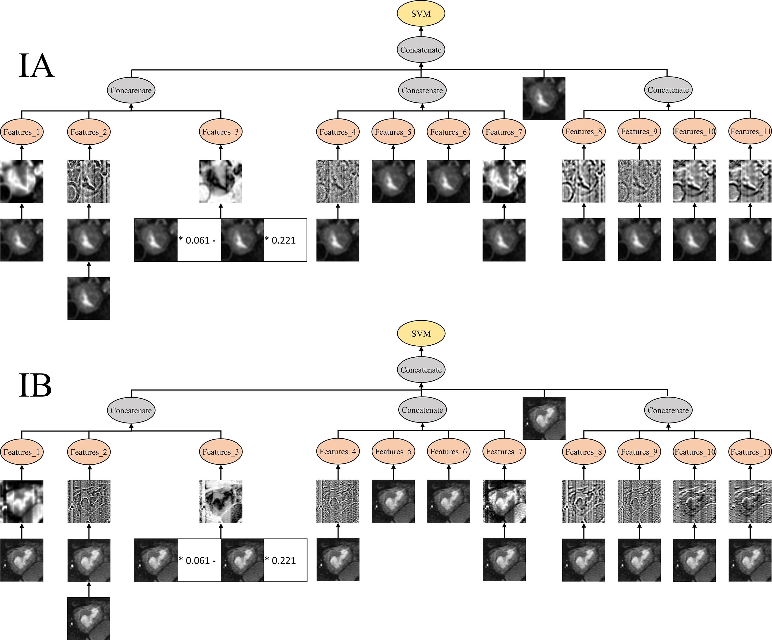 Fig. 9.
Features produced by the example program from different classes. The figure shows example images from stage IA and IB EC processed by the GP program. Image features were extracted using HOG, SIFT, and uLBP, concatenated to form high-level features, and classified using SVM and ERF with ensemble learning. Abbreviations: GP, genetic programming; HOG, Histogram of Oriented Gradients; SIFT, Scale-Invariant Feature Transform; uLBP, uniform Local Binary Patterns; SVM, Support Vector Machine; ERF, Extreme Random Forest. * denotes multiplication by a coefficient in the GP-derived expression.
This study evaluated a GP-based classification framework for distinguishing FIGO stage IA and IB endometrial cancer based on the automatic detection of ROIs in MRI images. The results obtained with this approach demonstrated high classification performance for distinguishing FIGO stage IA from IB across multiple MRI sequences. Specifically, the FELGP-based model achieved an accuracy of 0.92 and an AUC of 0.96 on the test set, while the FlexGP-based model achieved an accuracy of 0.87 and an AUC of 0.92. These results demonstrate the effectiveness and robustness of GP-based feature construction for the staging of early EC. Comparative results presented in Table 4 and Fig. 7 show that FlexGP and FELGP consistently outperform COGP and IDGP, which may be attributed to the design of their function sets. First, FlexGP and FELGP incorporate an additional filtering and pooling layer, enabling the extraction of more informative texture and structural features from MRI images. Second, FELGP further introduces ensemble learning strategies through classification and combination layers, allowing the integration of multiple classifiers and resulting in improved robustness. Performance differences across MRI sequences were also observed. Axial DWI achieved higher classification accuracy than sagittal T2WI, which can be explained by intrinsic modality characteristics. Although this study did not explicitly quantify image contrast or analyze GP features at the contrast level, DWI is clinically known to provide higher lesion-to-background contrast and greater sensitivity to tumor cellularity. The superior classification performance achieved on DWI therefore suggests that the discriminative patterns captured by the GP framework are more effectively represented in this modality, providing indirect evidence that DWI is more suitable for GP-based feature construction in early-stage EC classification. In contrast, sagittal T2WI images often contain more anatomical variability and may suffer from partial volume effects, increasing the difficulty of accurately distinguishing between stage IA and IB. Despite these challenges, the GP-based framework showed consistently competitive performance across modalities. From a computational perspective, GP-based feature construction is computationally expensive during training. However, all evolutionary optimization procedures are performed offline. During online inference, only ROI detection, evaluation of evolved GP expressions, and a single classifier prediction are required. This design enables near real-time inference and allows the proposed automated classification framework to provide objective decision-support information in clinical workflows, particularly during the preoperative staging of early-stage EC. Compared with existing methods, such as manually engineered feature-based ML models or CNN-based classifiers that require large training datasets, the proposed GP-based approach offers clear advantages in terms of small-sample learning and interpretability. Once trained, the model can make predictions using only a limited number of images, making it suitable for many real-world medical imaging scenarios where annotated data are scarce.
Despite the promising results, several limitations should be acknowledged. First, this study was conducted on a relatively small dataset collected from a single institution, which may limit the generalizability of the findings. Nevertheless, the primary aim of this work was to investigate the feasibility of GP-based classification under limited data conditions, which are common in medical imaging applications. Future studies will focus on validating the proposed framework using larger, multi-center datasets to assess robustness across different MRI scanners and acquisition protocols. Second, ROI images were used for GP-based classification. While ROI cropping improves classification accuracy and reduces the computational burden, it may lead to partial loss of tumor volume and spatial contextual information. Exploring strategies that incorporate more global spatial context is another potential direction for future research. Third, although different MRI modalities were evaluated independently in this study, multimodal feature fusion was not explored. Combining complementary information from DWI and T2WI within a unified GP framework has the potential to further improve staging performance. However, direct multimodal fusion would substantially increase the feature dimensionality and GP search space, which may increase the risk of overfitting under the current setting of limited samples. Future work with larger datasets and more efficient GP search strategies should investigate multimodal GP-based feature fusion to further enhance robustness and classification accuracy. Fourth, the general-purpose GP function sets in this study were intentionally adopted to maintain broad applicability and reduce the risk of overfitting under a small-sample setting. Although several existing GP classification algorithms were evaluated, no GP method was specifically designed for MRI image analysis. The development of domain-specific GP architectures and the incorporation of medical imaging–oriented function sets may further improve performance and interpretability. Finally, the reference labels used in this study were derived from clinician-confirmed, postoperative pathological staging, which served as the gold standard. Although preoperative MRI staging is routinely performed in clinical practice, structured and standardized radiologist-assigned MRI staging results were not consistently available in this retrospective dataset. In some cases, MRI reports contained descriptive assessments without explicit stage assignment, while in others, formal staging conclusions were not reported. Consequently, paired preoperative–postoperative staging outcomes could not be extracted reliably, and discrepancies between preoperative MRI staging and final pathological staging could not be quantitatively analyzed. Future work will involve the collection of more complete and standardized preoperative MRI staging reports, together with postoperative pathology. This will allow a systematic head-to-head comparison, enabling further evaluation of the clinical utility of the proposed GP-based classification framework.
In this paper, four GP-based algorithms were compared for the classification of stage IA and IB EC based on MRI images. The method first detects the ROI on raw MRI images using SSD object detection, followed by cropping of the ROI image. Feature extraction and construction from the cropped ROI images were subsequently performed using GP. Finally, the new features were used to train the stage IA and IB EC classifier, resulting in a highly accurate classification model. The proposed GP-based method was verified on three types of MRI images and compared to ML- and DL-based baseline methods. The results showed that cropped ROI images could improve classification accuracy and reduce computational costs. For medical images, the GP-based method did not require massive training data and avoided the requirement for essential rich domain knowledge after the image preprocessing stage. Furthermore, the model demonstrated a strong resistance to overfitting, evidenced by the marginal gap between training and testing accuracies, confirming its robustness in limited-data scenarios. In summary, this GP-based method can effectively classify stage IA and IB EC, thus providing a novel solution for medical image diagnosis with a small amount of data.
Data will be made available from the corresponding author on reasonable request.
CC: Writing - original draft, Resources, Project administration, Data curation. YS: Resources, Investigation, Methodology. WC: Resources, Validation, Formal analysis. JH: Validation, Software, Methodology, Data curation. ML: Software, Validation. YX: Visualization, Formal analysis. ZL: Investigation, Data curation. YL: Writing - review editing, Supervision, Conceptualization, Project administration, Funding acquisition. All authors contributed to editorial changes in the manuscript. All authors read and approved the final manuscript. All authors have participated sufficiently in the work and agreed to be accountable for all aspects of the work.
The Institutional Review Board (IRB) of Fujian Maternity and Child Health Hospital (FMCHH) in China approved our retrospective study (No. 2025KY166), and the requirement for informed consent was waived. The study was carried out in accordance with the guidelines of the Declaration of Helsinki.
Not applicable.
This study was supported by the Fujian Key Laboratory of Women and Children’s Critical Diseases Research (2024OP001) and the Guide Fund for the Development of Local Science and Technology from the Central Government (2023L3019).
The authors declare no conflict of interest.
References
Publisher’s Note: IMR Press stays neutral with regard to jurisdictional claims in published maps and institutional affiliations.