

 , Hui-Chen Lu 1, Zih-Han Wu 1, Tzu-Chi Chang 2
1 Department of Mathematics, National Chung Cheng University, 621301 Chiayi, Taiwan
2 Institute of Statistics, National University of Kaohsiung, 811 Kaohsiung, Taiwan
Abstract
Obesity is a chronic condition linked to health issues such as diabetes, heart disease, and increased cancer risk. High body mass index (BMI) is associated with cancers such as breast and colorectal cancer due to hormone imbalances and inflammation from excess fat, whereas a low BMI can raise cancer risk by weakening the immune system. Maintaining a normal BMI improves cancer treatment outcomes, but in some cases, higher BMI might offer protective effects—a phenomenon known as the “obesity paradox”. This study explores how BMI affects gene expression in cancer, using data from The Cancer Genome Atlas (TCGA), aiming to uncover links between BMI and cancer progression while identifying potential treatment targets.
To analyze the data, a two-stage method using overlapping group screening (OGS) was applied. First, gene groups were identified with the “grpregOverlap” R package. Then, their interactions were tested using the sequence kernel association test. Significant gene-gene interactions were selected based on statistical measures. In the second stage, predictive models were built using regularized regression techniques such as ridge regression, lasso, and adaptive lasso, with generalized ridge regression used to improve accuracy and stability in handling high-dimensional data.
The proposed OGS-based method was tested on simulated and real-world datasets. Results showed that combining OGS with generalized ridge regression and adaptive lasso (OGS_G.ridge_ALasso) gave the best prediction performance, with lower error rates and greater stability compared to other models like support vector regression, k-nearest neighbors, and random forests. In practical applications, gene expression and BMI data from TCGA patients (including bladder, cervical, esophageal and liver cancers) were integrated to identify key genes and interactions related to BMI.
Through evaluations on both simulated synthetic datasets and real-world datasets, we demonstrated the effectiveness of the proposed method in terms of predictive accuracy. Additionally, we identified BMI-associated genes and gene-gene interaction biomarkers across different cancer types and presented the corresponding network structures. Based on the key genes and gene interactions identified, we further explored how BMI influences cancer development and prognosis, providing deeper insights into the biological mechanisms underlying these associations.
Keywords
- body mass index
- gene-gene interaction
- overlapping group screening
- precision medicine
- regularized linear regression
- TCGA
According to the World Health Organization (WHO) in its report Obesity and Overweight, obesity is a chronic and multifaceted condition characterized by excessive fat accumulation that can negatively affect health. It increases the risk of developing conditions such as type 2 diabetes, heart disease and certain cancers. Obesity also impacts bone health, reproductive function, and can reduce quality of life by affecting sleep and physical activity levels [1]. The link between Body Mass Index (BMI) and cancer risk is a critical concern in the field of health. BMI, a metric calculated from a person’s height and weight, is commonly used to assess whether an individual is underweight, overweight, or at a healthy weight. The formula for calculating BMI is: BMI = weight (kg) / height (m)2. Both high and low BMI are associated with an increased risk of developing cancer.
A high BMI (overweight or obesity) increases the risk of several cancers including breast, colorectal, endometrial, esophageal and kidney cancers [2, 3, 4]. Excess fat alters hormone levels, such as androgens, estrogens and progesterone that can promote cancer growth [5]. It is also linked to insulin resistance and elevated insulin levels, further increasing cancer risk. Obesity triggers chronic inflammation and immune response changes that support cancer cell growth [6]. Conversely, low BMI (underweight) can increase cancer risk due to malnutrition and weakened immunity, making the body more susceptible to cancer while also being associated with digestive system cancers such as oral and gastric cancers [7]. Maintaining a healthy BMI (18.5–24.9) through a balanced diet and moderate exercise can therefore help reduce cancer risk.
BMI significantly affects the prognosis of cancer patients. Huang et al. [8] showed that a high BMI (obesity) is linked to poorer outcomes, with obese patients facing higher risks of complications, treatment failure and cancer recurrence, especially in breast and colorectal cancers. Obese patients also have higher mortality risks in cancers like uterine, colorectal, ovarian and liver cancers [7]. In contrast, underweight patients may experience malnutrition, weakened immunity, poor treatment tolerance and longer recovery, leading to shorter survival [9]. Maintaining a normal BMI (18.5–24.9) improves prognosis, with better treatment outcomes, lower recurrence and longer survival, as it supports immune function, reduces metabolic issues, and enhances treatment effectiveness.
Obese breast cancer patients, especially postmenopausal women, have a higher risk of recurrence after surgery [10]. Overweight and obese prostate cancer patients are at greater risk of postoperative recurrence and have lower survival rates [11] while further reducing treatment effectiveness and inducing more severe side effects [12]. Significant weight changes, whether loss or gain, can affect prognosis, particularly during chemotherapy, and markedly, excessive weight loss (cancer cachexia) is linked to poorer survival outcomes [13]. In conclusion, both high and low BMI are associated with worse cancer prognosis, while maintaining a normal BMI improves treatment outcomes and survival.
While obesity is traditionally seen as a carcinogen, it may have a protective effect in certain stages and types of cancer by enhancing antitumor immunotherapy. This challenges the view that obesity increases cancer mortality risk, known as the “Obesity Paradox”. The paradox suggests that overweight and Class 1 obese (BMI = 25–34.9) cancer patients may have a better prognosis than lean individuals, though this is not true for all patients or cancer types [14]. Studies like Tu et al. [15] found that although overweight or obesity increases the risk of developing cancer, among patients already diagnosed with cancer, having a slightly higher body weight around the time of diagnosis is associated with lower risk of death and longer survival, and this finding applies to most cancer types. Petrelli et al. [16] found that obese patients with cancers like renal cell carcinoma, lung cancer and melanoma may better tolerate chemotherapy and experience lower mortality rates.
Alifano et al. [17] studied the impact of preoperative BMI on survival in non-small cell lung cancer (NSCLC) patients undergoing lung resection, and determined that underweight patients had lower survival rates, while overweight and obese patients had better outcomes. For obese patients, a higher BMI was associated with improved survival, even after adjusting for various factors. In breast cancer, Modi et al. [18] found that a higher BMI worsened survival in early breast cancer (EBC) but improved survival in advanced breast cancer (ABC). In colorectal cancer, some studies linked obesity to a higher risk of death, while others showed that obese patients had longer survival and better treatment tolerance [19]. In summary, while obesity is generally associated with increased health risks, in certain cancer patients, a higher BMI may be linked to lower mortality, potentially due to factors like treatment tolerance, biological mechanisms, hormone levels and cancer subtypes.
This study used The Cancer Genome Atlas (TCGA) data to explore the relationship between BMI and gene expression. BMI, as an indicator of body fat, can influence various aspects of a cancer patient’s physiological condition, nutritional status and immune system. Abnormal BMI (either high or low) is often associated with biological changes that may affect gene expression, metabolic pathways, immune responses and more. By analyzing TCGA data, we can investigate the correlation between BMI and specific genes or gene clusters related to metabolism, inflammation, hormone regulation or cell proliferation, providing insights into how BMI impacts cancer development and prognosis. Additionally, genes interact to regulate processes like cell growth, death and migration, and studying such interactions between BMI-related genes can offer a more comprehensive understanding of how BMI influences cancer biology. For example, certain genes may collaborate in high BMI patients to drive cancer progression or influence treatment response. This research could uncover molecular mechanisms linking BMI to cancer and identify new targets or biomarkers to better understand how BMI affects cancer onset and prognosis.
We analyzed data from 1825 patients across seven TCGA cancer types to explore
BMI-associated molecular characteristics with details shown in Table 1. Due to
the small number of underweight cases (BMI
| Cancer Type | Number of Patients | Underweight (BMI |
Normal (BMI 18.5–25) | Overweight (BMI 25–30) | Obese (BMI |
| BLCA | 356 | 9 | 138 | 124 | 85 |
| CESC | 258 | 12 | 88 | 72 | 86 |
| COAD | 211 | 1 | 70 | 74 | 66 |
| COADREAD | 279 | 5 | 84 | 109 | 81 |
| ESCA | 175 | 8 | 89 | 49 | 29 |
| KIRP | 212 | 5 | 46 | 86 | 75 |
| LIHC | 334 | 21 | 156 | 89 | 68 |
BMI, Body Mass Index; BLCA, bladder urothelial carcinoma; CESC, cervical squamous cell carcinoma and endocervical adenocarcinoma; COAD, colon adenocarcinoma; COADREAD, colorectal adenocarcinoma; ESCA, esophageal carcinoma; KIRP, kidney renal papillary cell carcinoma; LIHC, liver hepatocellular carcinoma.
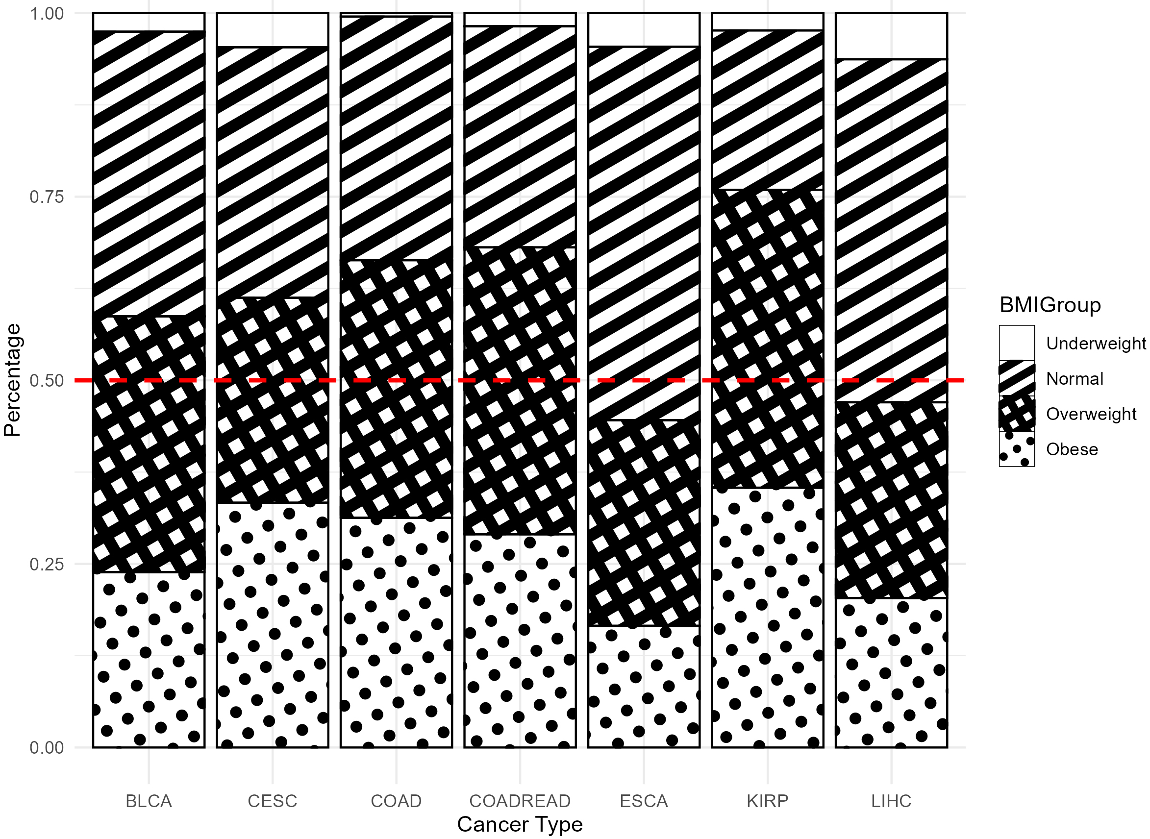
As shown in Fig. 1, over 60% of patients in most cancer types had a BMI
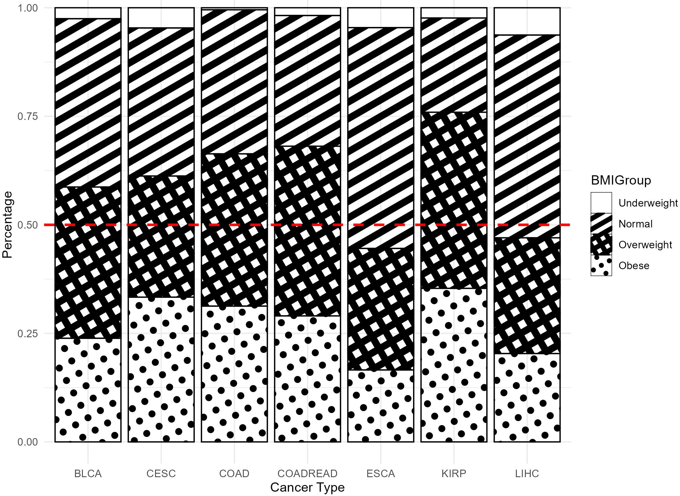 Fig. 1.
Proportion of four BMI groups across different cancer types. BMI, Body Mass Index.
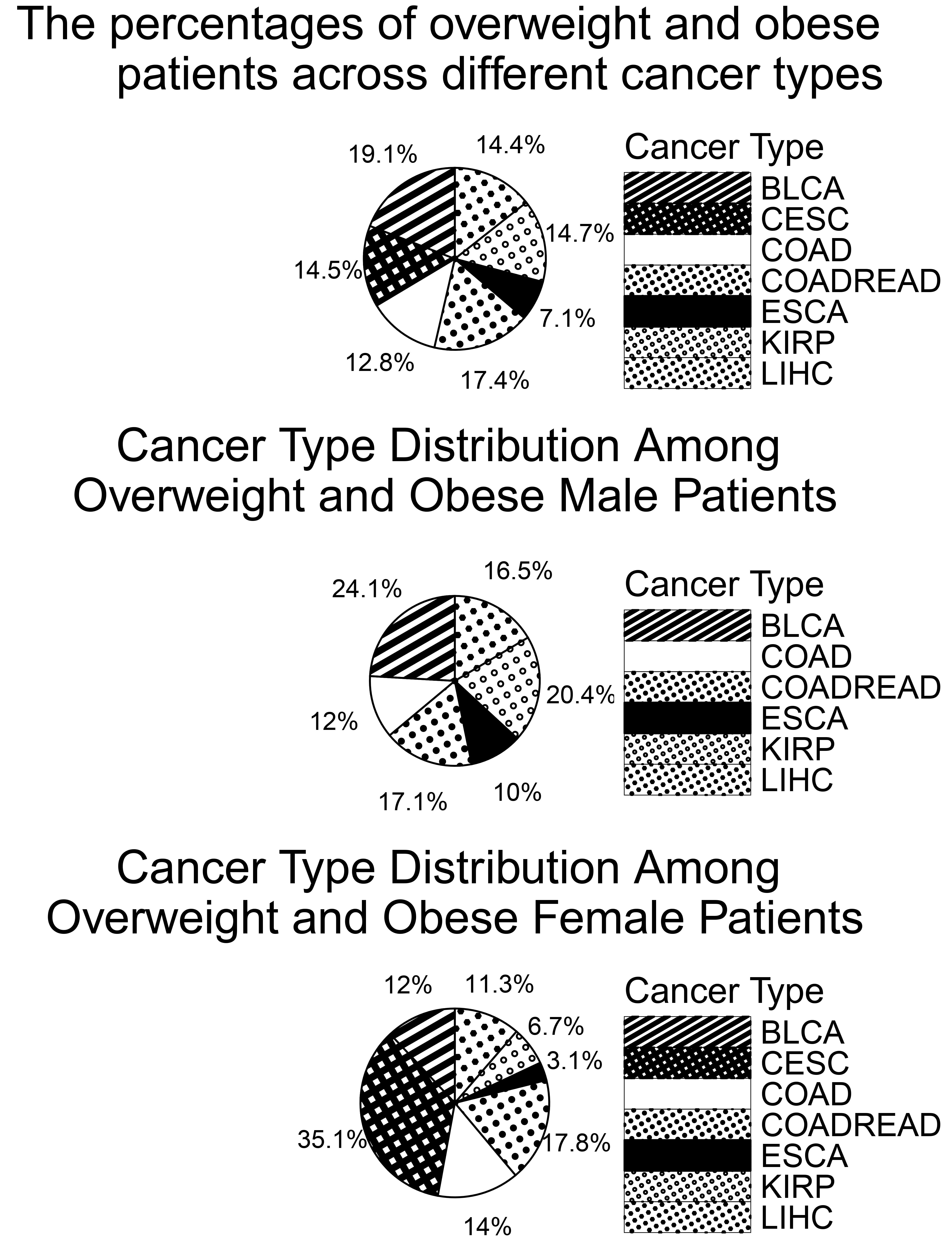
Fig. 2 (top) shows the distribution of overweight and obese patients across cancer types, totaling 1093 individuals. BLCA had the highest number (209 patients, 19.1%), while ESCA had the lowest (78 patients, 7.1%), consistent with the previously noted lower BMI trend in ESCA. Patients were also grouped by sex: 750 females and 1075 males. As shown in Fig. 2 (middle), BLCA was the most common cancer type among overweight and obese males. Based on these findings, we further examined BMI-related gene expressions in BLCA and CESC. In Fig. 2 (bottom), CESC had the highest proportion among overweight and obese females. This supports findings by Clarke et al. [21], which suggest that overweight and obese women face a higher risk of CESC, potentially due to under-diagnosis of precancerous lesions.
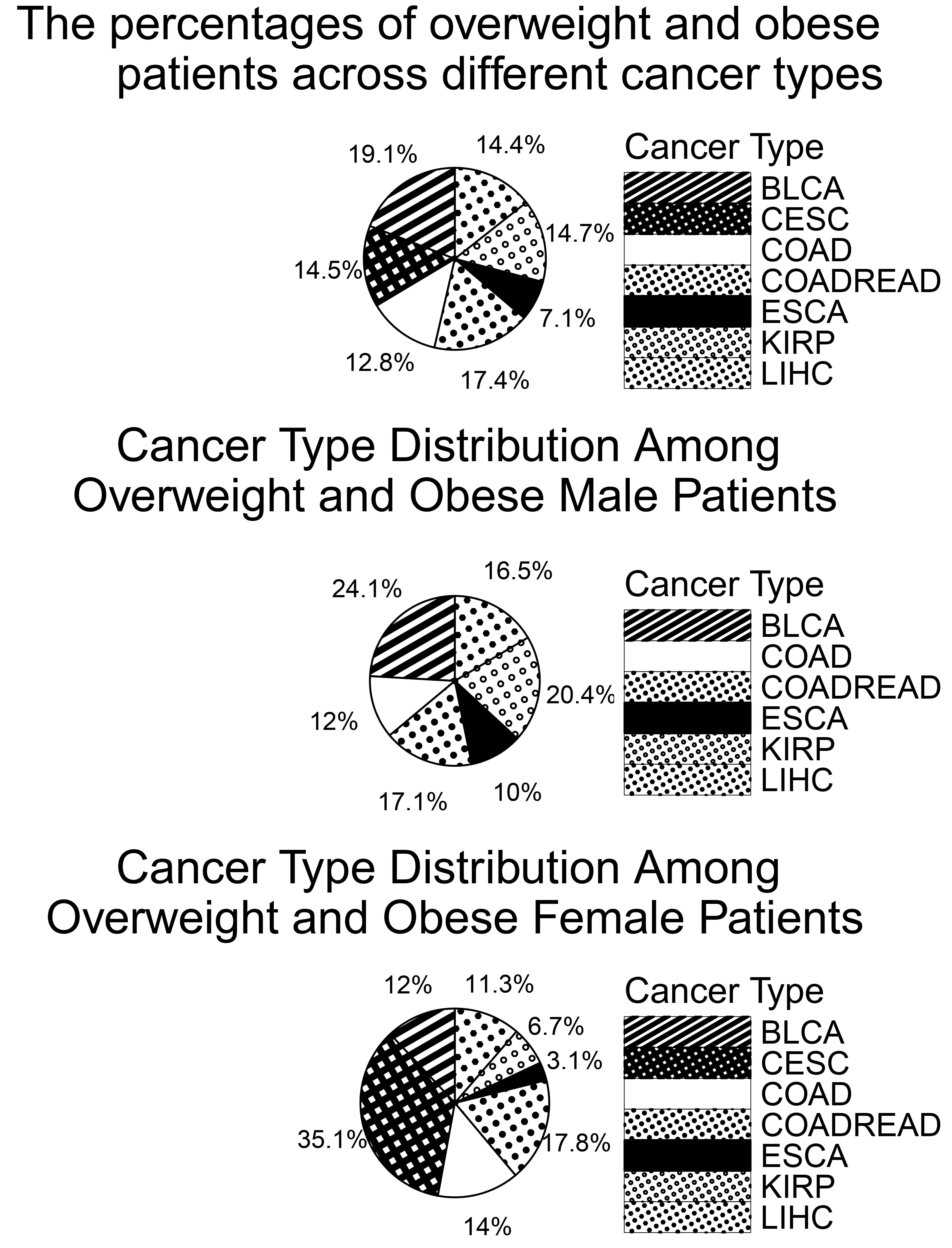 Fig. 2.
Percentage of overweight and obese patients by cancer type and gender.
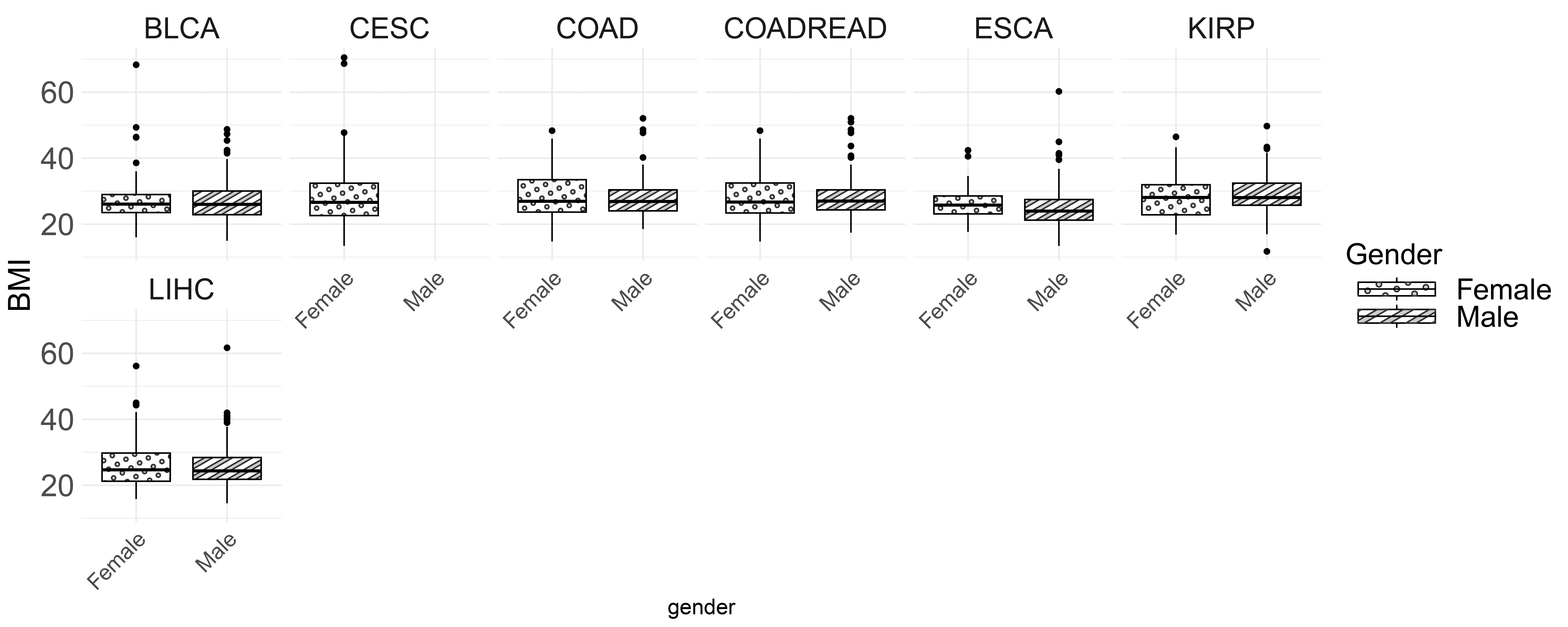
Fig. 3 shows the BMI distribution for male and female patients across various cancer types. The boxplot highlights the median BMI, interquartile range (IQR) and outliers. Generally, the median BMI is similar for both genders, except in BLCA and KIRP, where males have slightly higher BMIs. In COAD, COADREAD and ESCA, females have a slightly higher median BMI. Additionally, CESC shows greater BMI variability, suggesting more significant differences among patients.
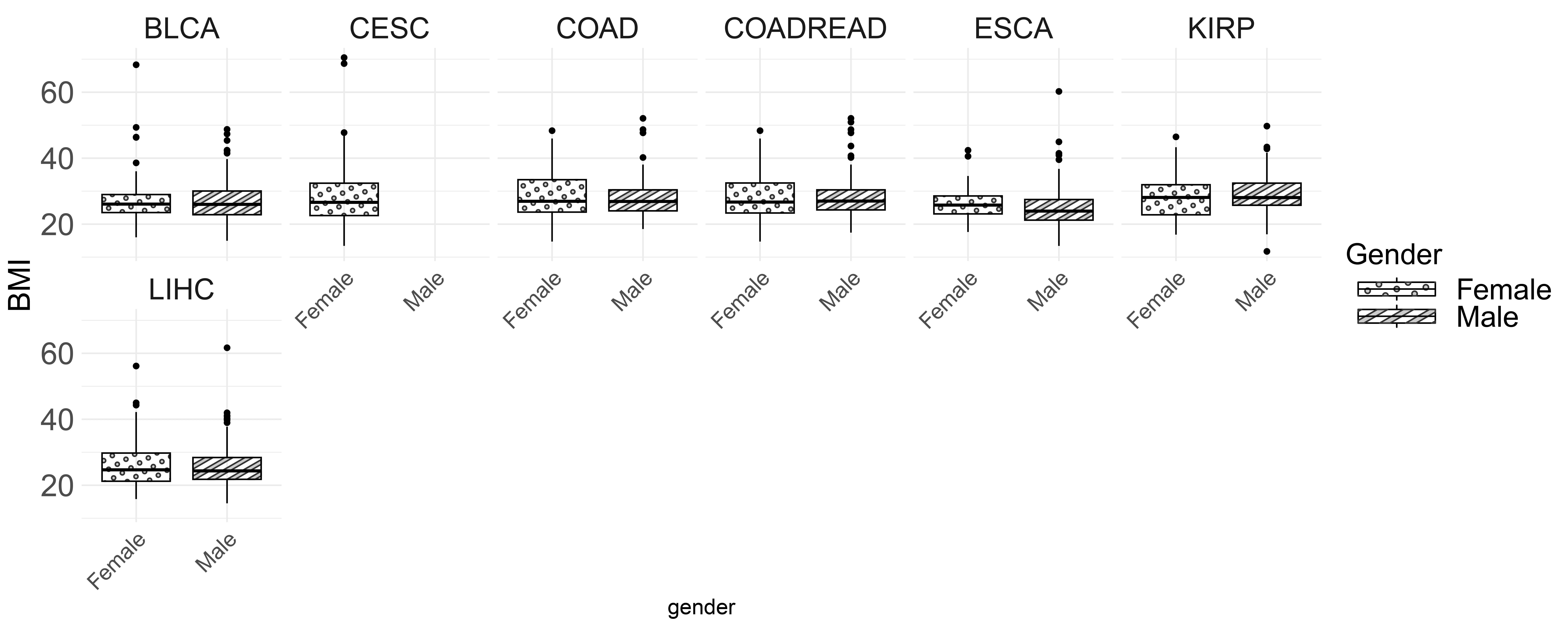 Fig. 3.
BMI distribution by gender and cancer type.
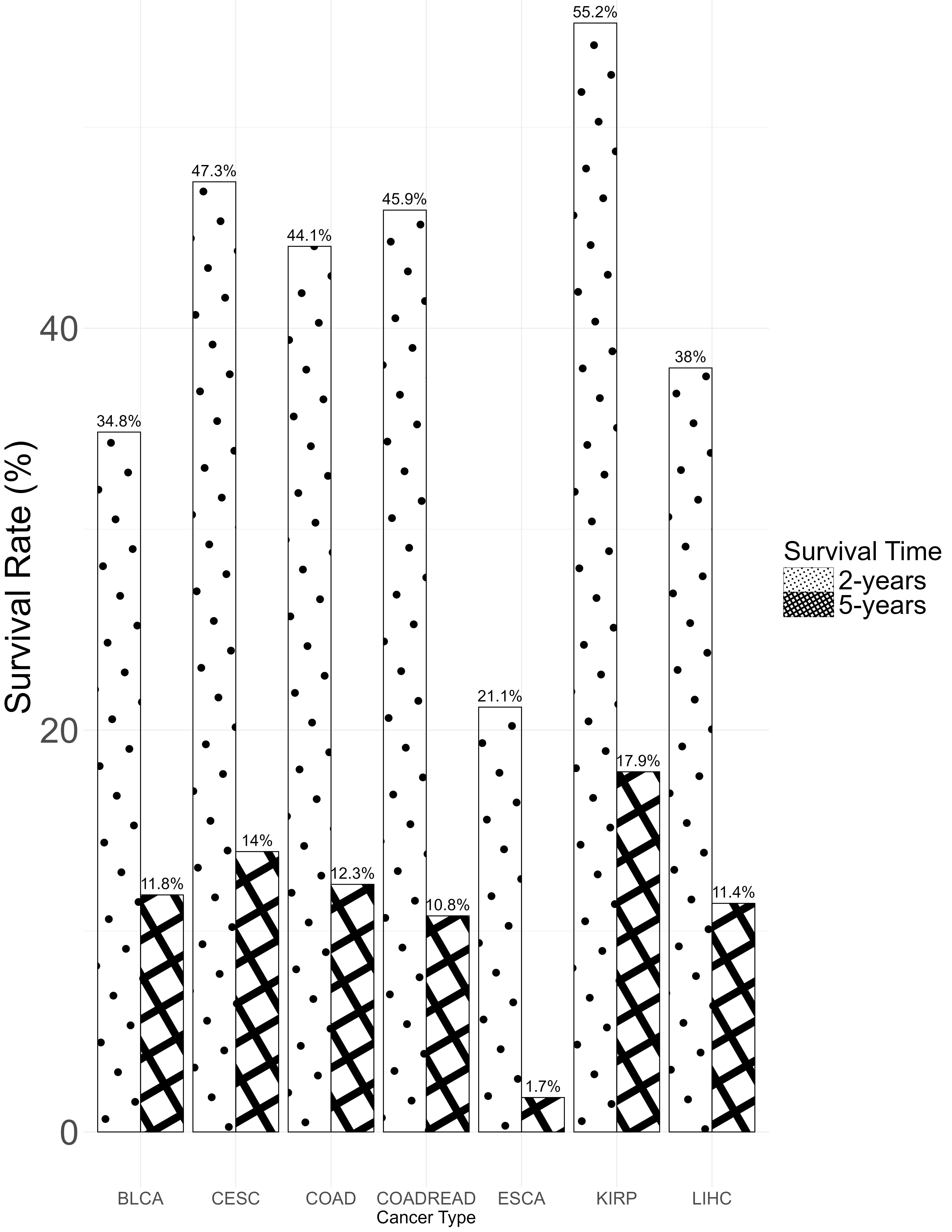

Fig. 4 displays the two-year and five-year survival rates for patients across different cancer types. Except for ESCA and LIHC, which have lower obesity rates, other cancer types with higher obesity proportions have a two-year survival rate above 35%, some exceeding 55% (e.g., KIRP), while five-year survival rate differences are less pronounced. Fig. 5 shows Kaplan-Meier survival curves for each BMI category (normal, overweight, obese), with a log-rank test p-value of 0.001, indicating a significant survival difference between the groups where overweight and obese groups have higher survival rates than the normal group.
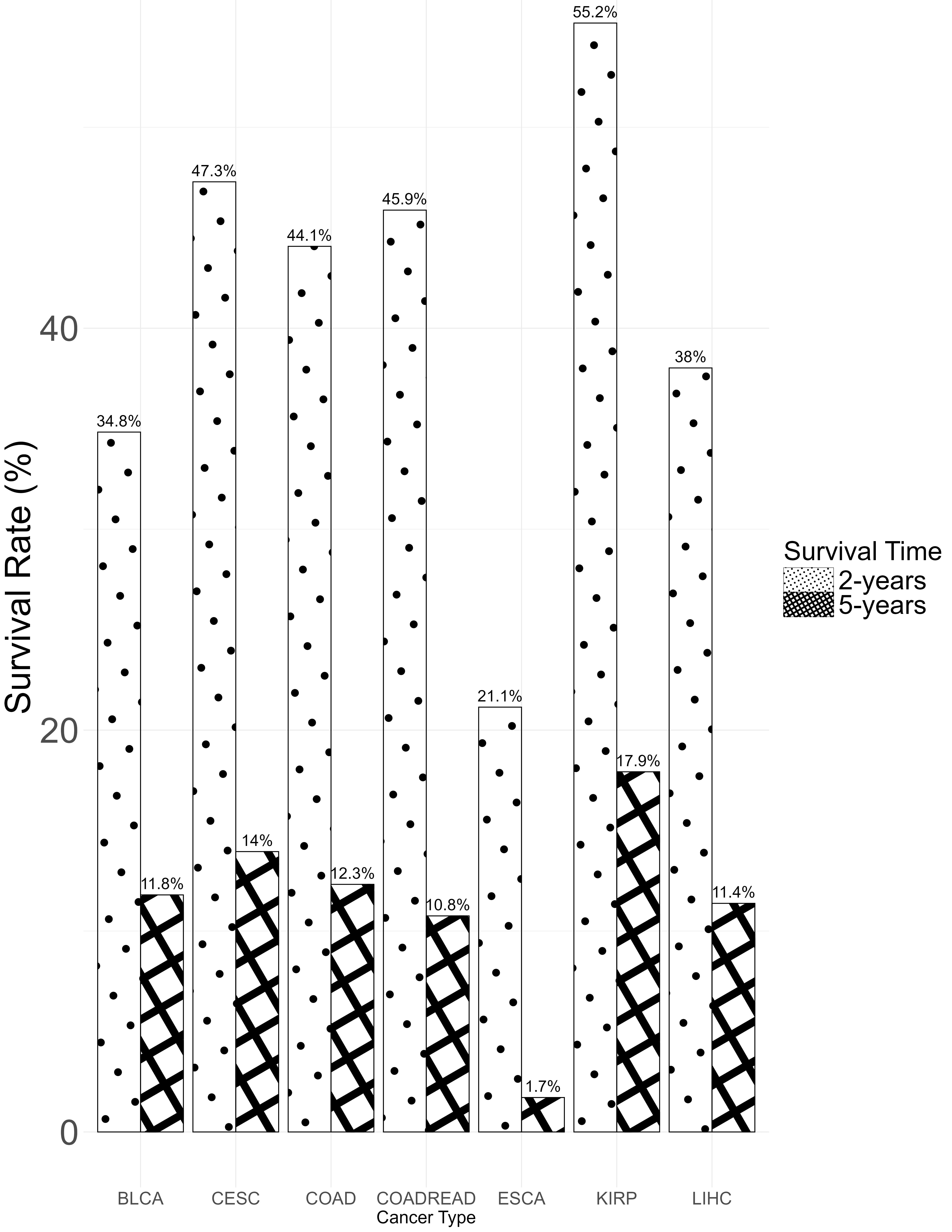 Fig. 4.
Two-year and five-year survival rates by cancer type.
 Fig. 5.
Kaplan-Meier survival curves by BMI group.
We conducted a Cox regression analysis using the three BMI categories (normal, overweight and obese) as a categorical variable, adjusting for age and gender. Table 2 shows the coefficient estimates, p-values and hazard ratios for BMI (overweight) and BMI (obesity) across seven cancer types with results indicating that, except for BLCA and ESCA, the coefficient estimates for BMI (overweight) and BMI (obesity) were mostly negative, suggesting a lower risk of death with higher BMI. Specifically, negative and statistically significant coefficients for BMI (obesity) were seen in COAD, COADREAD and the combined data, while the coefficient for BMI (overweight) was also negative and significant for the combined data.
| Cancer Type | Number of Patients | Censoring rate | Coef (p-value) of BMI_overweight | Coef (p-value) of BMI_obesity |
| All DATA | 1825 | 0.7200 | –0.2307 (0.0223) | –0.4190 (0.0003) |
| BLCA | 356 | 0.5787 | 0.2539 (0.1760) | –0.0461 (0.8341) |
| CESC | 258 | 0.7984 | –0.5499 (0.1429) | –0.3802 (0.2326) |
| COAD | 211 | 0.8009 | –0.0657 (0.8402) | –1.3015 (0.0182) |
| COADREAD | 279 | 0.8029 | –0.0869 (0.7681) | –0.7899 (0.0567) |
| ESCA | 175 | 0.6000 | –0.0514 (0.8601) | 0.2367 (0.4470) |
| KIRP | 212 | 0.8585 | 0.0251 (0.9580) | –0.2200 (0.6640) |
| LIHC | 334 | 0.6647 | –0.3190 (0.1730) | –0.2047 (0.4090) |
In summary, this study analyzed 1825 patients from seven TCGA cancer types to investigate the relationship between BMI, cancer characteristics and prognosis. Most patients were overweight or obese except for those with ESCA and LIHC, likely due to weight loss related to disease symptoms. Among high-BMI patients, bladder cancer (BLCA) was most common in males, and cervical cancer (CESC) in females. Higher BMI was generally associated with better two-year survival rates. Kaplan-Meier and Cox regression analyses indicated that, except for BLCA and ESCA, higher BMI was linked to a lower risk of death in most cancer types.
Although the Kaplan–Meier curves indicate that overweight and obese patients had significantly better survival rates (p = 0.001), the Cox regression results varied across cancer types. The non-significant findings in BLCA and ESCA might be due to limited sample sizes (particularly in ESCA), tumor heterogeneity, or the lack of clinical information such as treatment details and comorbidities in the TCGA dataset. It is also important to note that the Kaplan–Meier analysis reflects unadjusted survival differences, while the Cox model adjusts for variables such as age and gender, so such adjustment might dilute the effect of BMI, especially in cancer types where these covariates have a strong impact on prognosis. Caution should therefore be exercised when interpreting the relationship between BMI and survival.
We conducted a study with n subjects, each with genetic data
represented by a vector of p genes
TCGA transcriptomic data were obtained using the R package “UCSCXenaTools” [23], while genomic data for TCGA BLCA, LIHC, ESCA and CESC used in this study were available from the TCGA Hub on the UCSC Xena platform (https://tcga.xenahubs.net). For example, the TCGA BLCA dataset comprised 365 patients with recorded height and weight measurements, along with gene expression profiles covering 20,501 genes per individual. BMI was derived from the height and weight data.
To compare the performance of regression models, the study used several performance metrics from the R package “Metrics” such as Min-Max Accuracy, mean absolute percentage error (MAPE), symmetric mean absolute percentage error (SMAPE), root mean squared error (RMSE), mean absolute scaled error (MASE), mean absolute error (MAE) and median absolute error (MDAE). The definitions are as follows:
Among these metrics, only Min-Max Accuracy favors values close to 1, indicating better model performance; for all others, so smaller values imply fewer errors and better predictions. Each metric suits different contexts: RMSE emphasizes larger errors and is suitable when extreme errors matter, while MAE provides a general average error size. MDAE, based on the median, is more robust to outliers and useful when extreme values exist. MASE is common in time series analysis, allowing comparison across different scales. MAPE and SMAPE express errors as percentages; however, MAPE can become unstable when actual values near zero, while SMAPE mitigates this through symmetric treatment. Studies [24] highlight MAPE’s bias toward low predictions, making it less reliable in some cases. SMAPE, introduced to address MAPE’s limitations, is gaining popularity due to its balanced error expression [25, 26]. Thus, this study focuses on SMAPE results. In summary, selecting the right metric based on data traits is crucial for meaningful model evaluation.
This study applied overlapping group screening (OGS) to identify gene and
interaction biomarkers related to quantitative phenotypes. OGS has been widely
used in genomics, addressing outcomes such as censored survival time [27], binary
tissue classification [28] and multinomial cancer subtype classification [29].
The method uses a two-stage group screening to detect both main and interaction
effects. Since gene pathways can overlap, the latent effect model by Jacob
et al. [22] is adopted to handle shared genes across groups. All
transcriptomic data must be standardized before applying OGS. The procedure of
the OGS method for linear regression models
Step 1: To identify biologically relevant gene sets (i.e., pathways), we began by applying the overlapping group binary logistic regression framework, implemented via the R package “grpregOverlap” [30]. This approach enables simultaneous feature selection while accommodating gene membership in multiple functional groups.
Step 2: Building on the strategy proposed by Wang and Chen [27], we generated sets of gene-gene (G-G) interaction pairs, which fall into three categories: interactions occurring within a single candidate pathway, interactions spanning two distinct candidate pathways identified in Step 1, and interactions linking one selected pathway with a previously uncharacterized pathway. For each group of G-G interactions, we evaluated its association with the quantitative trait using the Sequence Kernel Association Test (SKAT) [31]. This test yields a group-level p-value by aggregating the effects of individual interactions through a weighted sum of chi-square distributions. The p-values are derived using the Davies method [32], implemented in the “CompQuadForm” R package [33]. A lower p-value signifies stronger evidence for association and thus higher relevance in downstream analysis. Interaction groups are retained for model development if their p-values fall below a predetermined threshold.
Step 3: Finally, incorporating the selected pathways and interaction groups, we constructed a predictive model for BMI based on microarray data. This is achieved through regularized linear regression methods, including ridge regression, lasso [34] and adaptive lasso [35], as implemented in the “glmnet” R package [36]. We also provided a detailed description of the OGS method, including its mathematical formulation, underlying assumptions (such as group sparsity and gene overlap), and the associated optimization procedure, with full details presented in the Supplementary Material.
Regularized regression controls model complexity by adding a penalty term to the objective function, aiming to prevent overfitting, improve generalization, and identify key variables in high-dimensional data. It extends ordinary least squares (OLS) by penalizing both large and small regression coefficients to reduce overfitting and model complexity. Common methods include ridge (L2), lasso (L1) and adaptive lasso. Adaptive lasso builds on ridge estimates to reduce multi-collinearity, then uses their absolute values in a weighted lasso penalty, increasing the chance of shrinking unimportant coefficients to zero and selecting the most relevant features.
According to the study by Hoerl and Kennard [37], the objective function of the ridge regularized linear regression model is as follows:
The vector
According to the study by Tibshirani [34], the objective function of the linear regression model with lasso (least absolute shrinkage and selection operator) is as follows:
The vector
Adaptive lasso is an improved regularization method of lasso, primarily aimed at overcoming the issue of selection inconsistency in lasso and enhancing the accuracy of variable selection. The core idea is to introduce weights into the penalty term of lasso, adjusting the penalty based on the importance of the variables. According to Zou [35], the objective function of adaptive lasso is as follows:
The vector
In high-dimensional data (where p
where λ > 0 is the shrinkage parameter, and
where
The optimal
where
Finally, the generalized ridge regression estimator is defined as
In addition,
Generalized ridge regression can be implemented using the R package “g.ridge”. Emura et al. [39] showed through simulations and real data that it outperforms traditional ridge regression. They recommend standardizing predictors and excluding an intercept term; thus, the response variable Y should be centered by subtracting its mean. This study uses estimates from generalized ridge regression as initial weights for Adaptive Lasso, aiming to enhance prediction performance.
In our machine learning (ML) pipeline, we begin by utilizing the OGS method to pinpoint key gene biomarkers and interaction signals that will serve as features for downstream predictive modeling.
To construct regression-based prediction models, we explore several algorithms. For support vector regression (SVR), we adopt a radial basis function kernel. Hyperparameter tuning is performed for the “Cost” parameter across a wide logarithmic scale: 10-2, 10-1, 1, 101, …,105, including 0, and for the “Epsilon” parameter across values from 0.0 to 1.0 in 0.1 increments. This grid search and model evaluation are carried out using the tune function from the “e1071” R package, which performs cross-validation to identify the optimal SVR configuration. For the k-nearest neighbors (KNN) algorithm, we employ a rectangular kernel and use the kknn function from the “kknn” package. The number of neighbors is tuned within a range of 1 to 50 through cross-validation, seeking the value that yields the best predictive accuracy. Within the Random Forest (RF) modeling framework, two key hyperparameters are optimized: the number of trees, evaluated across values from 1 to 500, and the number of features considered at each split, explored over a range from 1 to d/3, where d denotes the number of features [40]. This tuning process is implemented using the randomForest and tuneRF functions from the “randomForest” R package, again relying on cross-validation to determine the configuration that offers the best generalization performance.
In the following simulations, we evaluate the predictive performance of the proposed OGS method combined with regularized regression or machine learning models, and compare it to Oracle, sure independence screening (SIS) Lasso and Ordinary Lasso methods. The Oracle method uses the true underlying model, which is known in simulations but not in real-world cases. SIS Lasso first ranks genes and gene-gene (G-G) interactions using univariate regression, selects the top n / (2 * log (n)) predictors, and applies lasso regression to build the final model. Ordinary Lasso directly applies lasso regression to all genes and G-G interactions without preselection.
To demonstrate the effectiveness of the proposed OGS-based feature selection combined with regularized linear regression, we perform a comprehensive numerical study. This analysis not only highlights the behavior of our approach under controlled conditions but also benchmarks its predictive accuracy against a set of well-established machine learning algorithms. A synthetic dataset comprising 300 simulated observations is employed for training purposes. Each individual response is generated from an underlying linear regression framework, ensuring a structured ground truth for model comparison,
with the covariates
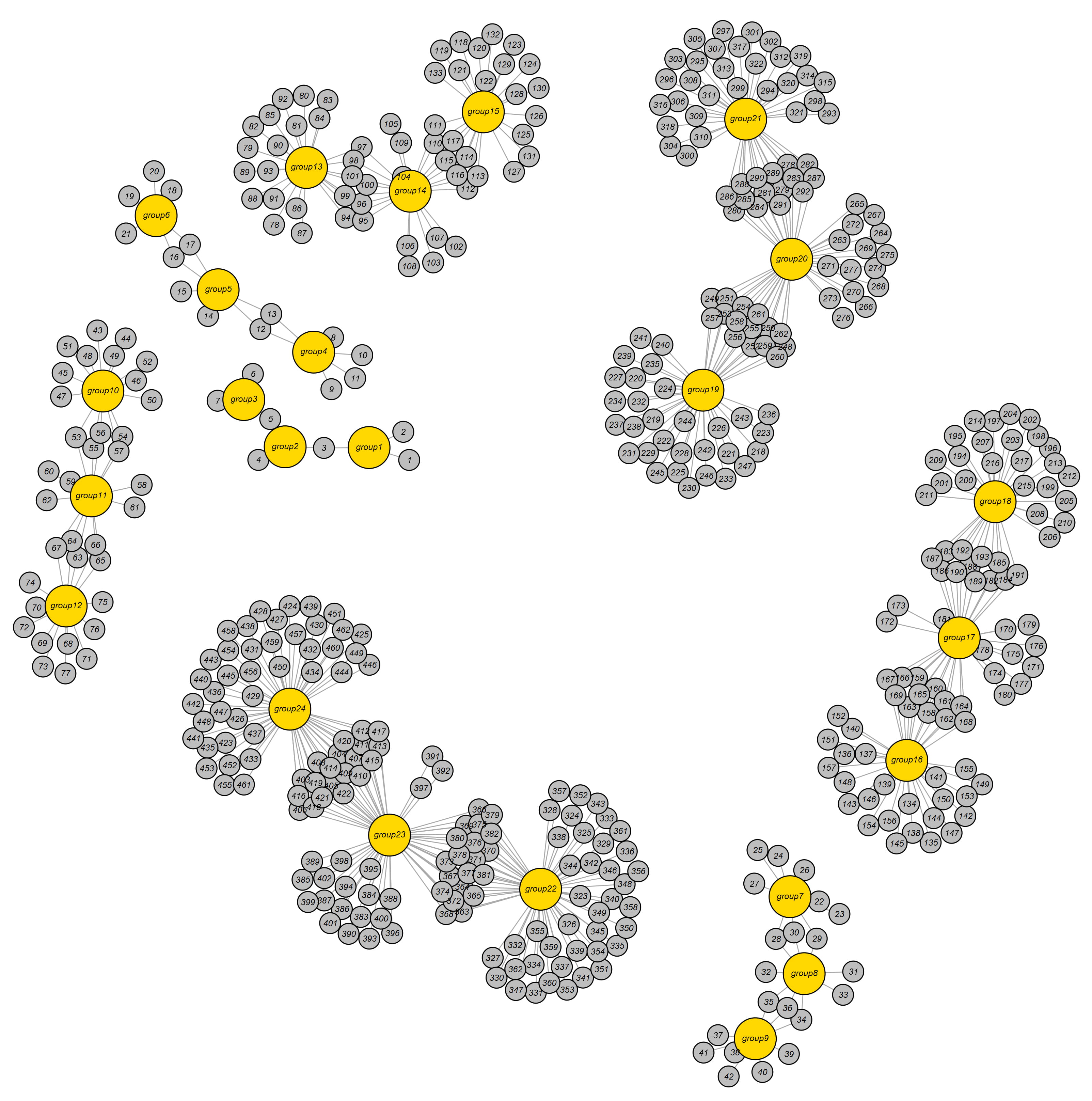
The simulation considers both gene group size and overlapping structure, as illustrated in Fig. 6. For example, groups 10 and 11 each contain 15 genes, sharing 5 genes and totaling 25 unique ones. In total, the study includes 462 genes and 594 group-specific gene effects. Groups 1, 7, 13 and 19 are set to have significant effects, with constant values of 2.25, 2.25, 1.5 and –1.5 respectively. In group 13, key gene-gene interactions (G78–G90, G80–G88, G82–G86) have coefficients of 4, 6 and 4. For groups 13 and 7, interactions (G23–G81, G24–G83, G25–G85) have coefficients 4, 6 and 4.8. The simulation includes 106,953 major gene and G-G interaction pairs.
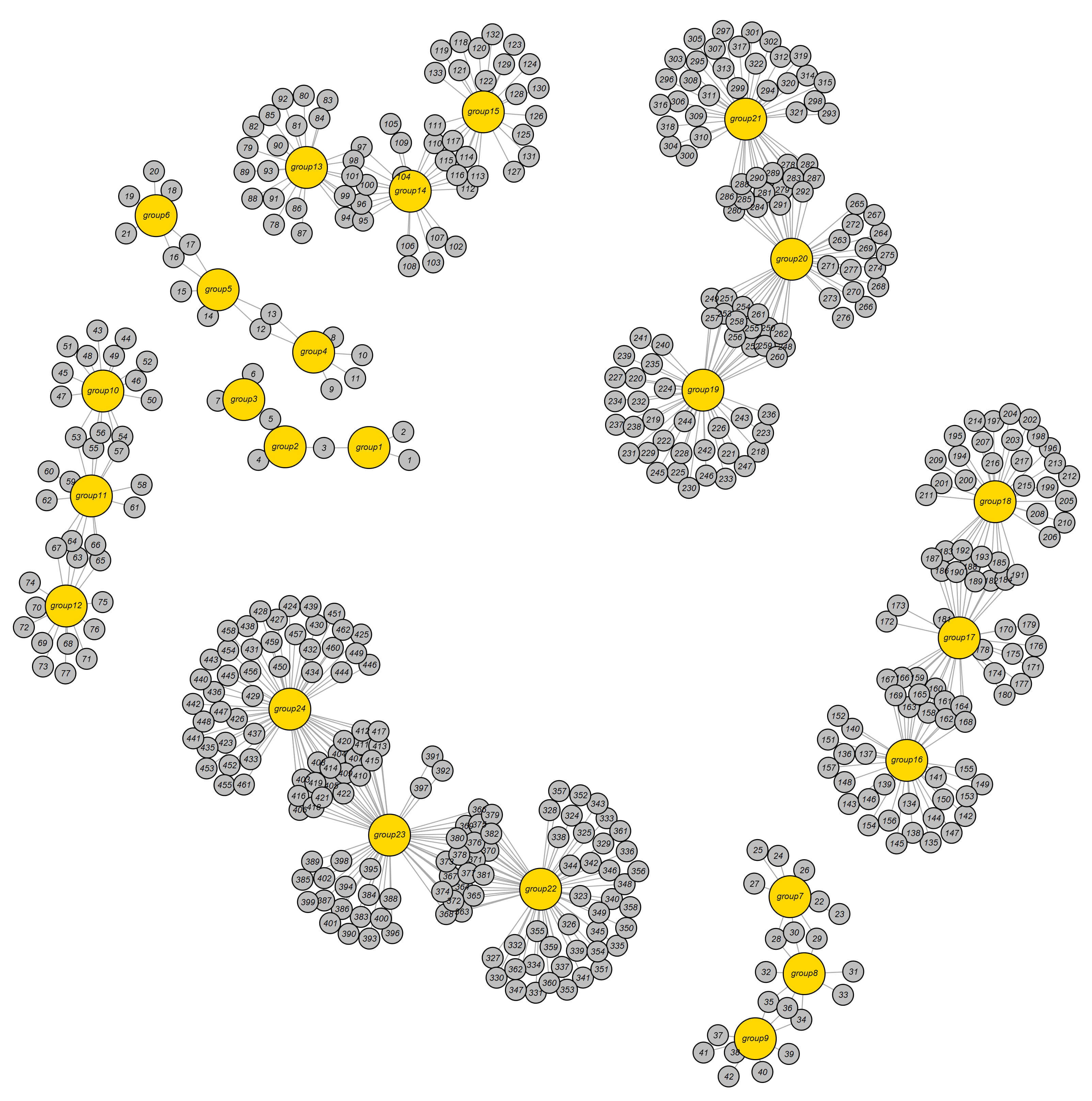 Fig. 6.
The gene network structure for the varying gene group-size data.
We conducted the simulation 200 times to obtain numerical results. As shown in Table 3, the OGS method with ridge, lasso and adaptive lasso penalties consistently outperformed other methods, including standard ML techniques. Notably, OGS_G.ridge_ALasso achieved the best SMAPE performance, averaging 96.4460% with a standard deviation of 13.1026%, indicating both low prediction error and high stability. This highlights its strong advantage in high-dimensional prediction tasks.
| Method | MinMax Accuracy | MAPE (%) | SMAPE (%) | RMSE | MASE | MAE | MDAE |
| Oracle | 1.0686 (0.7929) | 53.4438 (102.1502) | 22.0822 (3.9587) | 3.5935 (0.2577) | 0.0584 (0.0070) | 2.8536 (0.2212) | 2.3782 (0.2798) |
| SIS_Lasso | 2.0543 (10.7865) | 297.4343 (975.8890) | 124.8943 (7.1654) | 36.1921 (2.6755) | 0.5898 (0.0505) | 28.9182 (2.1914) | 24.5015 (2.7976) |
| Ordinary_Lasso | 74.5814 (1037.1391) | 209.2237 (210.6191) | 107.6245 (7.0998) | 29.8888 (2.4651) | 0.4877 (0.0449) | 23.9117 (1.9552) | 20.2449 (2.2624) |
| OGS_Ridge | –1.2573 (55.1990) | 251.0337 (499.1449) | 139.1917 (7.7979) | 39.8240 (3.2943) | 0.6458 (0.0497) | 31.7181 (2.7719) | 26.7102 (3.2483) |
| OGS_Lasso | –0.0528 (9.5304) | 246.4983 (244.9423) | 98.7028 (12.9678) | 27.7523 (4.1344) | 0.4535 (0.0730) | 22.2170 (3.3410) | 18.9009 (3.0896) |
| OGS_ALasso | 1.3383 (6.1393) | 286.5519 (617.4884) | 100.2347 (11.4929) | 29.0729 (4.6024) | 0.4748 (0.0796) | 23.2607 (3.6681) | 19.8310 (3.4925) |
| OGS_G.ridge | –0.4462 (9.7117) | 311.3224 (526.7253) | 121.4321 (13.3355) | 36.8617 (5.1348) | 0.5973 (0.0856) | 29.3041 (4.1555) | 24.7078 (4.3394) |
| OGS_G.ridge_ALasso | 0.7357 (2.5986) | 244.8488 (198.9061) | 96.4460 (13.1026) | 27.5813 (5.2893) | 0.4507 (0.0914) | 22.0708 (4.2530) | 18.7724 (3.9844) |
| OGS_SVR | –2.2300 (48.6514) | 164.9359 (255.0762) | 139.3309 (12.5035) | 37.2596 (3.6611) | 0.6008 (0.0537) | 29.5154 (2.9300) | 24.5860 (3.0880) |
| OGS_RF | 0.6033 (9.7192) | 299.7391 (1442.5547) | 129.8464 (8.2173) | 37.0854 (2.9283) | 0.6019 (0.0482) | 29.5477 (2.4636) | 24.9841 (2.8997) |
| OGS_KNN | 21.5828 (253.5380) | 202.8519 (538.8489) | 159.9890 (10.0371) | 42.7823 (3.1866) | 0.6945 (0.0490) | 34.1005 (2.6264) | 28.7858 (3.2589) |
MAPE, mean absolute percentage error; SMAPE, symmetric mean absolute percentage error; RMSE, root mean squared error; MASE, mean absolute scaled error; MAE, mean absolute error; MDAE, median absolute error; SIS, sure independence screening; OGS, overlapping group screening; SVR, support vector regression; RF, Random Forest; KNN, k-nearest neighbors.
Compared to other ML methods like OGS_RF, OGS_SVR and OGS_KNN, OGS_G.ridge_ALasso shows significantly higher accuracy. OGS_KNN (SMAPE: 159.9890%) and OGS_SVR (SMAPE: 139.3309%) have large fluctuations, indicating poor stability and adaptability. Even against the relatively strong OGS_Lasso, OGS_G.ridge_ALasso performs better across multiple metrics, including SMAPE, Min-Max Accuracy, MAE and MDAE, demonstrating more balanced predictive performance.
While both OGS_G.ridge and OGS_Ridge are based on ridge regression, OGS_G.ridge uses a generalized version that adjusts penalty strength based on variable characteristics, offering more flexibility. It achieves nearly 18% lower SMAPE than OGS_Ridge. Despite a slightly higher standard deviation, its improved accuracy suggests that generalized ridge better captures complex data relationships. Comparing OGS_ALasso with OGS_G.ridge_ALasso shows further improvement when generalized ridge is introduced. Both use adaptive lasso for variable selection, but OGS_G.ridge_ALasso applies variable-specific penalties, aiding in retaining key information. Though the SMAPE improvement is about 3.8%, it remains meaningful in complex high-dimensional data.
In conclusion, OGS_G.ridge_ALasso shows clear advantages over traditional ridge, adaptive lasso and other ML methods, offering low error and high stability. It is especially effective for high-dimensional structured problems like genetic data, highlighting both theoretical progress and practical potential.
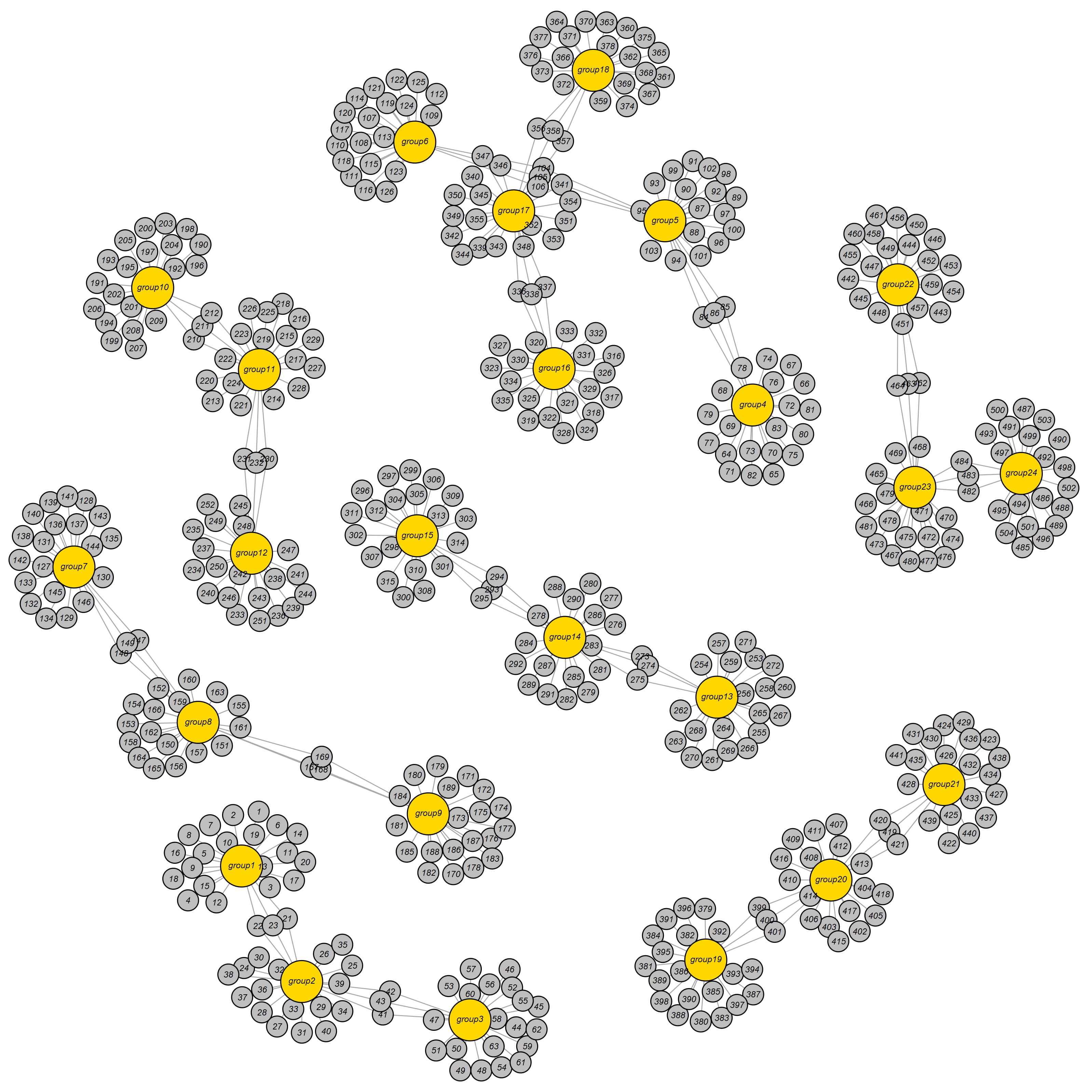
We also examine an alternative gene network with 24 groups, each containing 23 genes, detailed in Fig. 7. This setup includes 504 genes and 552 group-specific gene effects. Groups 1, 7, 13 and 19 have significant effects, with underlying values of 2.25, 2.25, 1.5 and –1.5 respectively. In group 13, key gene-gene interactions (G253–G265, G255–G263, G257–G261) have coefficients 4, 6 and 4. For groups 13 and 7, interactions (G128–G266, G130–G268, G132–G270) have coefficients 4, 6 and 4.8. The simulation includes 127,260 major gene and interaction pairs.
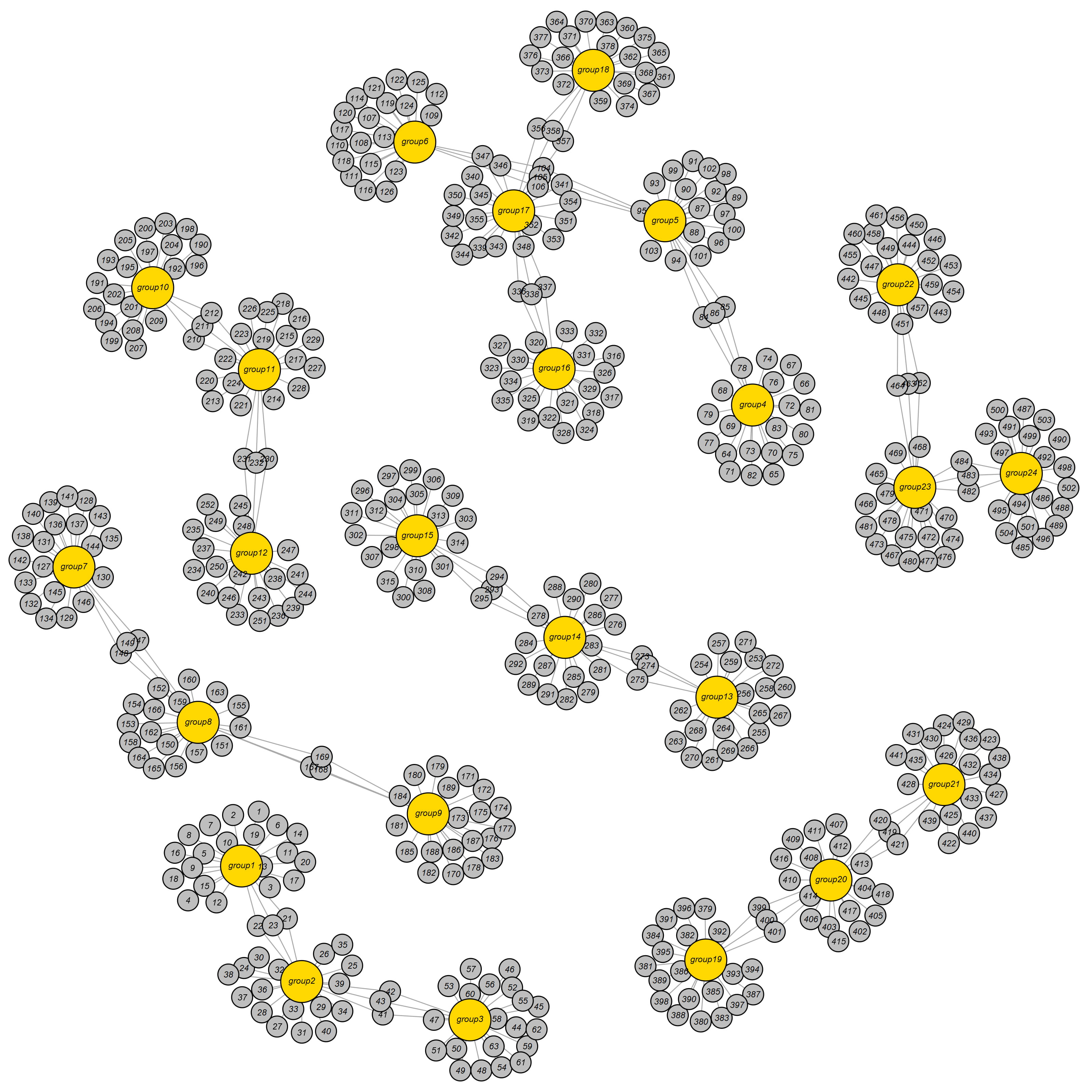 Fig. 7.
The gene network structure for the equal gene group-size data.
According to Table 4, OGS_G.ridge_ALasso achieved the best predictive performance among all models, with an average SMAPE of 114.8411% and a standard deviation of 13.7029%, indicating both low error and high stability—making it well-suited for high-dimensional structured data. In contrast, most machine learning methods showed higher SMAPE values, likely due to overfitting or difficulty capturing the underlying data structure.
| Method | MinMax Accuracy | MAPE (%) | SMAPE (%) | RMSE | MASE | MAE | MDAE |
| Oracle | 1.1878 (2.6650) | 64.1145 (262.2200) | 20.3052 (3.6218) | 3.6105 (0.2804) | 0.0530 (0.0062) | 2.8617 (0.2415) | 2.3847 (0.3062) |
| SIS_Lasso | 1.5922 (16.2790) | 325.4094 (698.8159) | 133.8282 (8.1499) | 42.9855 (3.1250) | 0.6353 (0.0469) | 34.4168 (2.6477) | 29.0987 (3.4569) |
| Ordinary_Lasso | –0.2268 (40.7950) | 258.2261 (649.2819) | 122.9424 (8.4288) | 37.7662 (2.8756) | 0.5580 (0.0428) | 30.2318 (2.4826) | 25.6980 (2.9641) |
| OGS_Ridge | 2.4615 (35.0658) | 299.4902 (855.1537) | 142.4277 (8.0232) | 44.8423 (3.2134) | 0.6610 (0.0478) | 35.8121 (2.7630) | 30.2960 (3.7008) |
| OGS_Lasso | 0.3925 (11.9970) | 371.0417 (963.1335) | 120.0683 (16.1679) | 38.3600 (4.9675) | 0.5683 (0.0821) | 30.7230 (4.0444) | 26.1716 (4.1695) |
| OGS_ALasso | 0.3897 (16.5750) | 456.8200 (1075.6511) | 118.0533 (12.8660) | 40.4871 (6.2626) | 0.5995 (0.1025) | 32.3873 (5.0111) | 27.5544 (4.6994) |
| OGS_G.ridge | –3.1482 (77.8741) | 502.7925 (1899.9081) | 128.0602 (10.9844) | 44.2214 (4.2306) | 0.6526 (0.0729) | 35.3018 (3.5517) | 29.8727 (4.0881) |
| OGS_G.ridge_ALasso | 2.1295 (22.2190) | 518.4625 (2103.3653) | 114.8411 (13.7029) | 39.2424 (6.7836) | 0.5824 (0.1121) | 31.4421 (5.4566) | 26.6852 (4.9976) |
| OGS_SVR | –0.4871 (28.2289) | 190.9094 (549.3813) | 137.7514 (17.4938) | 40.2370 (4.8160) | 0.5911 (0.0704) | 32.0259 (4.0320) | 26.8084 (4.3726) |
| OGS_RF | 3.5606 (50.9942) | 251.7642 (637.7145) | 140.2724 (10.7404) | 43.2332 (3.1884) | 0.6378 (0.0452) | 34.5680 (2.7642) | 29.4925 (3.4944) |
| OGS_KNN | –7.1837 (101.0930) | 283.6388 (1342.6511) | 157.5052 (11.5435) | 46.4494 (3.4574) | 0.6850 (0.0468) | 37.1275 (2.9458) | 31.4680 (3.5750) |
Compared to OGS_Lasso, OGS_G.ridge_ALasso improved SMAPE by about 5% and outperformed in other metrics, showing greater stability and predictive power. The addition of adaptive lasso to OGS_G.ridge further enhanced accuracy, significantly reducing SMAPE. This highlights the substantial performance gain achieved by combining the two techniques. OGS_Ridge, which lacks flexible variable selection, had relatively poorer performance. Similarly, OGS_G.ridge_ALasso outperformed OGS_ALasso (SMAPE = 118.0533%), highlighting the benefit of incorporating generalized ridge.
To further evaluate the robustness of the proposed method, we conducted an additional simulation study for sensitivity analysis. This analysis incorporated two different gene group structures (high-overlap and low-overlap scenarios) and simulated varying effect sizes by reducing the magnitude of the true biomarker coefficients (original coefficients divided by 2). Our results (Supplementary Tables 2,3) show that OGS_G.ridge_ALasso accurately identifies the relevant gene groups under these conditions, demonstrating strong robustness to varying signal strengths.
In summary, OGS_G.ridge_ALasso stands out in both accuracy and stability across metrics. It is particularly well-suited for high-dimensional and structurally complex prediction tasks, such as those involving genomic data, and holds significant practical value for real-world applications.
Given the potential contamination and batch effects in TCGA transcriptomic data, we performed data normalization during the preprocessing stage to minimize the impact of technical variability. Furthermore, to account for the possible presence of outliers, we employed the non-parametric Kendall’s tau correlation coefficient to identify the top 1000 genes significantly associated with BMI for subsequent analyses as this method is less sensitive to outliers, thereby enhancing the overall robustness of the analysis.
Our TCGA CESC dataset includes 258 subjects: 100 with BMI
We used a validation set approach, randomly splitting the dataset into 80% training (206 samples) and 20% testing (52 samples), and repeated this process 30 times after excluding 419 unmapped genes. Table 5 summarizes the average prediction results for BMI. We also evaluated two additional GO pathway databases: Biological Process (GO-BP) and Molecular Function (GO-MF) with results in Supplementary Tables 4,5. Across all databases, OGS_G.ridge_ALasso outperformed other methods, including standard machine learning models, particularly in terms of SMAPE, while also showing strong results in other metrics.
| MinMax Accuracy | MAPE (%) | SMAPE (%) | RMSE | MASE | MAE | MDAE | |
| SIS_Lasso | 0.8958 (2.9121) | 312.5154 (163.7632) | 148.5368 (9.3349) | 1.0794 (0.1569) | 0.8367 (0.1119) | 0.8275 (0.0903) | 0.6896 (0.1008) |
| Ordinary_Lasso | 7.2680 (49.3375) | 107.2105 (8.3599) | 185.2941 (8.9152) | 0.9095 (0.1420) | 0.7270 (0.0702) | 0.7215 (0.0729) | 0.6427 (0.0902) |
| OGS_Ridge | 1.5766 (4.2834) | 290.0074 (161.4077) | 140.2715 (10.2328) | 0.9688 (0.1473) | 0.7488 (0.0860) | 0.7420 (0.0788) | 0.6151 (0.0933) |
| OGS_Lasso | 0.4340 (4.8077) | 326.0319 (196.3179) | 138.4399 (10.0905) | 1.0091 (0.1454) | 0.7796 (0.0929) | 0.7717 (0.0755) | 0.6446 (0.0692) |
| OGS_ALasso | 0.0650 (5.3114) | 327.7718 (202.5703) | 138.0082 (10.0865) | 1.0106 (0.1478) | 0.7795 (0.0962) | 0.7713 (0.0768) | 0.6365 (0.0767) |
| OGS_G.ridge | 1.8217 (6.2966) | 291.1387 (164.8034) | 140.6525 (10.0384) | 0.9715 (0.1476) | 0.7516 (0.0866) | 0.7452 (0.0822) | 0.6079 (0.0888) |
| OGS_G.ridge_ALasso | 3.2068 (15.9334) | 329.9966 (208.0807) | 138.2342 (9.9804) | 1.0133 (0.1522) | 0.7810 (0.0965) | 0.7729 (0.0789) | 0.6429 (0.0750) |
| OGS_SVR | 1.2924 (3.4622) | 278.4534 (138.8284) | 142.9585 (9.0704) | 0.9415 (0.1428) | 0.7349 (0.0702) | 0.7299 (0.0792) | 0.6125 (0.0921) |
| OGS_RF | –4.0286 (25.6163) | 250.5968 (111.9902) | 144.7685 (9.8766) | 0.9288 (0.1457) | 0.7292 (0.0714) | 0.7248 (0.0866) | 0.6141 (0.0931) |
| OGS_KNN | –9.9220 (52.9677) | 267.7436 (129.7886) | 144.7497 (8.8615) | 0.9379 (0.1416) | 0.7343 (0.0715) | 0.7293 (0.0808) | 0.6136 (0.0926) |
The table reports the mean (standard deviation) of the test prediction performance for various prediction methods.
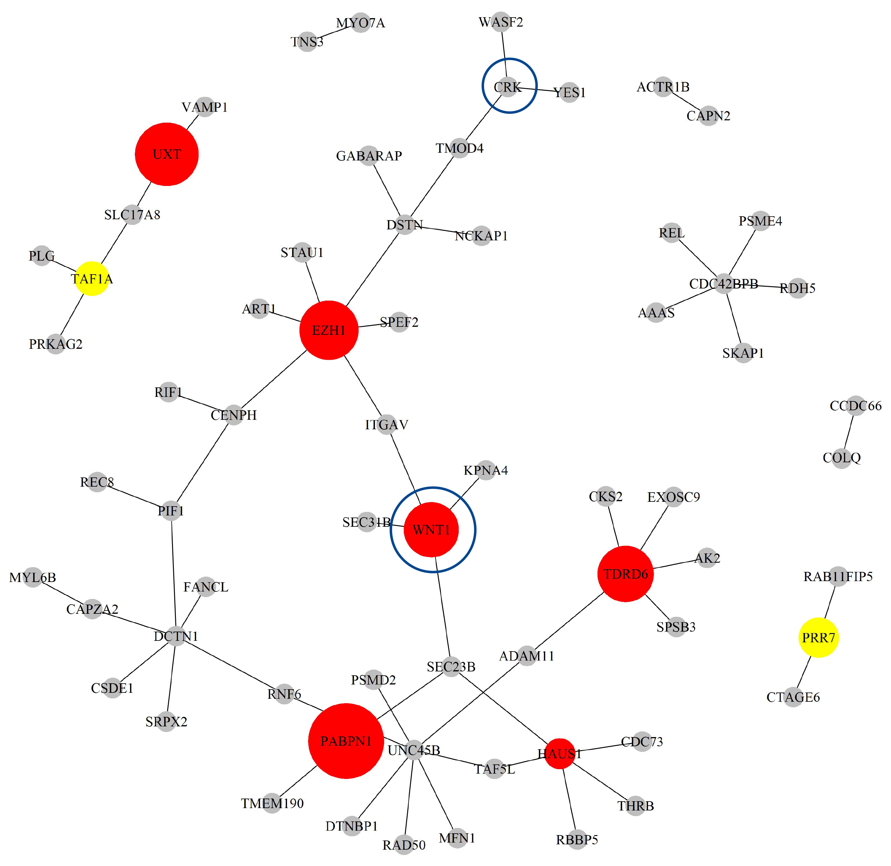
Next, based on the GO-CC pathway database, we apply our proposed method to the entire TCGA CESC dataset for model selection and parameter estimation. The method identifies 11 genes and 60 gene-gene interaction biomarkers, with corresponding network structure shown in Fig. 8 and and the top 10 highest and bottom 10 lowest biomarker coefficient values in shown in Table 6. Supplementary Table 6 presents all the selected biomarkers and their corresponding coefficients. In summary, we have incorporated node sizes and edge weight elements into the network figures. Larger nodes represent genes with greater importance. Additionally, the color of each node indicates the direction of effect: red represents a positive effect, while yellow represents a negative effect.
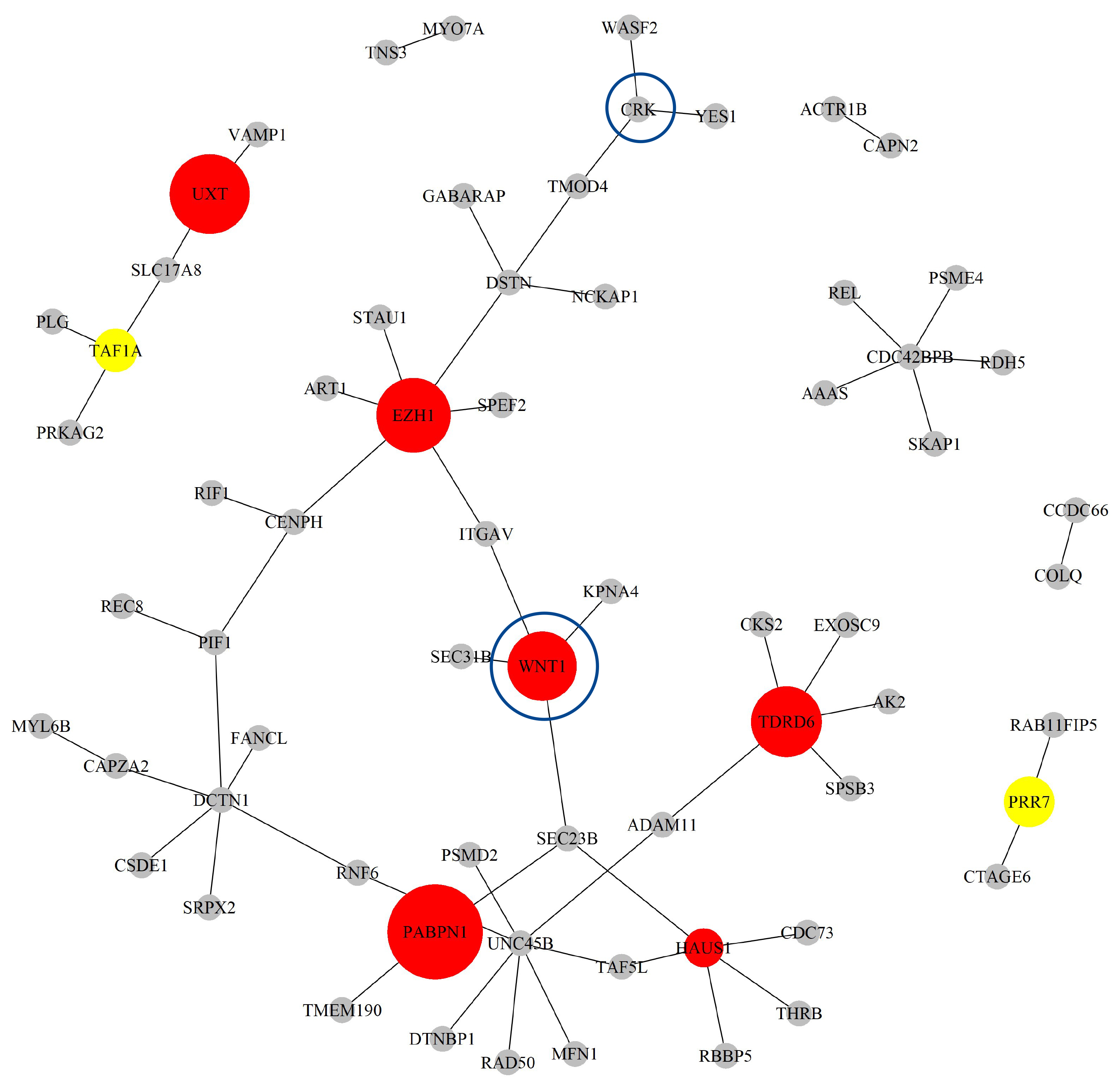 Fig. 8.
The Network structure of the selected G-G interaction by the proposed OGS_G.ridge_ALasso method in CESC.
| CESC (71 ACTIVE) | BLCA (42 ACTIVE) | LIHC (148 ACTIVE) | ESCA (71 ACTIVE) | ||||
| ID | Coefficient | ID | Coefficient | ID | Coefficient | ID | Coefficient |
| Top 10 biomarkers | |||||||
| SLC17A8-UXT | 0.1643 | C8A | 0.1287 | FUT5-GPR174 | 0.1549 | C15ORF48 | 0.1944 |
| EZH1-STAU1 | 0.1433 | C1QL2 | 0.1271 | FUT5-KCNB1 | 0.1439 | CATSPERB-IQCE | 0.1674 |
| PABPN1 | 0.1344 | LMOD2 | 0.1186 | PIGR | 0.1389 | ACE-DYNC1I1 | 0.1605 |
| CDC42BPB-PSME4 | 0.1241 | GYPB | 0.0975 | FUT5-PIGR | 0.1190 | IQCA1-SMO | 0.1443 |
| UXT | 0.1044 | MIOS | 0.0850 | FUT5-ZAP70 | 0.1189 | CALM3-SLC6A7 | 0.1416 |
| ADAM11-TDRD6 | 0.095 | ATP6V1B1 | 0.0766 | OPN4 | 0.1163 | SLC26A3-SLC3A2 | 0.1353 |
| EZH1 | 0.094 | ZFYVE1 | 0.0748 | ITGAX-SLC24A4 | 0.1117 | CALM3-LGALS3 | 0.1347 |
| EZH1-SPEF2 | 0.0929 | HPR-LMOD2 | 0.0623 | FUT5-RABEPK | 0.1031 | ITPKA | 0.1207 |
| DPF3 | 0.0913 | LILRA4 | 0.0618 | PPP3R2 | 0.0983 | CALM3-KIAA1614 | 0.1115 |
| TDRD6 | 0.0867 | INTS10-LMOD2 | 0.0589 | FPR2-FUT5 | 0.0976 | AQP2-ATP8A1 | 0.1091 |
| Bottom 10 biomarkers | |||||||
| CRK-TMOD4 | –0.1473 | DNAI2 | –0.1826 | CAT-FUT5 | –0.1342 | KIF9-SLC26A3 | –0.1892 |
| PLG-TAF1A | –0.1097 | EXOC7-HDAC1 | –0.1439 | FPR2-SLC24A4 | –0.1278 | ACE-CYS1 | –0.1372 |
| DEFA1B | –0.1052 | PPP1R3A | –0.1414 | HYAL3 | –0.1263 | CYS1-TTLL6 | –0.1347 |
| DTNBP1-UNC45B | –0.1020 | LMOD2-TRIOBP | –0.1217 | PLEC | –0.1210 | KIF3C-SLC26A3 | –0.1287 |
| DCTN1-FANCL | –0.1005 | LMOD2-OGDH | –0.0917 | HDAC6-PPP3R2 | –0.1156 | FXR1 | –0.1141 |
| SEC31B-WNT1 | –0.0919 | TRAPPC2 | –0.0863 | DCLRE1C | –0.1113 | CYS1-HYDIN | –0.1003 |
| ART1-EZH1 | –0.0913 | HDAC1 | –0.0845 | CHRAC1-FUT5 | –0.1093 | KIF9-TTLL6 | –0.0943 |
| PSMD2-UNC45B | –0.0774 | LMOD2-MAFG | –0.0771 | FUT5-UGT3A1 | –0.1087 | DYNLRB2-RSPH1 | –0.0834 |
| SLC17A8-TAF1A | –0.0664 | NME7 | –0.0745 | B4GALT2-PCSK6 | –0.1004 | MCM5 | –0.0738 |
| MFN1-UNC45B | –0.0642 | LMOD2-YAP1 | –0.0656 | FUT5-OS9 | –0.0996 | CALM3-CD44 | –0.0609 |
Some of the selected biomarkers have been confirmed to have biological
significance in existing literature. For example, Li et al. [41]
indicated that WNT1 is a target gene of miR-34a, and the decreased
expression of miR-34a (suppressed by HPV E6/E7) leads to an increase in
WNT1 expression. In CESC, WNT1 promotes cell proliferation,
invasion, and the conversion of “E-cadherin to P-cadherin” by activating the
WNT/
Our TCGA BLCA dataset includes 356 subjects: 147 with BMI
We used a validation set approach, randomly splitting the dataset into 80% training (284 samples) and 20% testing (72 samples), and repeated this process 30 times after excluding 380 unmapped genes. Table 7 summarizes the average prediction results for BMI. We also evaluated two additional GO pathway databases: GO-BP and GO-MF with results in Supplementary Tables 7,8. Across all databases, OGS_G.ridge_ALasso outperformed other methods, including standard machine learning models, particularly in terms of SMAPE, while also showing strong results in other metrics.
| MinMax Accuracy | MAPE (%) | SMAPE (%) | RMSE | MASE | MAE | MDAE | |
| SIS_Lasso | 6.2230 (20.4867) | 153.1523 (50.3734) | 159.6510 (7.2171) | 0.9784 (0.1658) | 0.7713 (0.0589) | 0.7357 (0.0815) | 0.6031 (0.0909) |
| Ordinary_Lasso | –28.3685 (87.3431) | 106.9705 (9.2948) | 182.0108 (12.8869) | 0.9494 (0.1656) | 0.7526 (0.0529) | 0.7179 (0.0780) | 0.5748 (0.0583) |
| OGS_Ridge | –0.9903 (8.9542) | 168.7948 (46.0440) | 151.4469 (13.4424) | 0.9629 (0.1597) | 0.7568 (0.0633) | 0.7211 (0.0750) | 0.5750 (0.0800) |
| OGS_Lasso | –0.3793 (5.0655) | 210.1537 (79.8495) | 144.6220 (13.9201) | 0.9877 (0.1588) | 0.7773 (0.0752) | 0.7393 (0.0714) | 0.6166 (0.0908) |
| OGS_ALasso | 11.8011 (74.5594) | 248.9250 (104.9382) | 139.6349 (10.3840) | 1.0477 (0.1979) | 0.8150 (0.1017) | 0.7732 (0.0774) | 0.6290 (0.0902) |
| OGS_G.ridge | –0.1931 (4.2451) | 229.5899 (84.3647) | 139.8774 (11.1173) | 1.0367 (0.2182) | 0.7929 (0.1018) | 0.7533 (0.0867) | 0.6097 (0.0904) |
| OGS_G.ridge_ALasso | –0.4559 (4.3949) | 280.6450 (149.6607) | 139.6553 (9.7535) | 1.0764 (0.1856) | 0.8329 (0.0967) | 0.7913 (0.0845) | 0.6418 (0.1015) |
| OGS_SVR | 0.4392 (4.4815) | 160.9705 (52.2773) | 147.9144 (13.6778) | 0.9469 (0.1701) | 0.7366 (0.0640) | 0.7025 (0.0811) | 0.5654 (0.0816) |
| OGS_RF | 4.2248 (14.5991) | 156.4021 (30.3354) | 156.6699 (8.4587) | 0.9722 (0.1473) | 0.7741 (0.0712) | 0.7360 (0.0669) | 0.6155 (0.0762) |
| OGS_KNN | –0.3208 (4.8648) | 171.0956 (58.5580) | 153.2306 (13.2028) | 0.9564 (0.1602) | 0.7586 (0.0676) | 0.7225 (0.0769) | 0.5925 (0.0829) |
The table reports the mean (standard deviation) of the test prediction performance for various prediction methods.
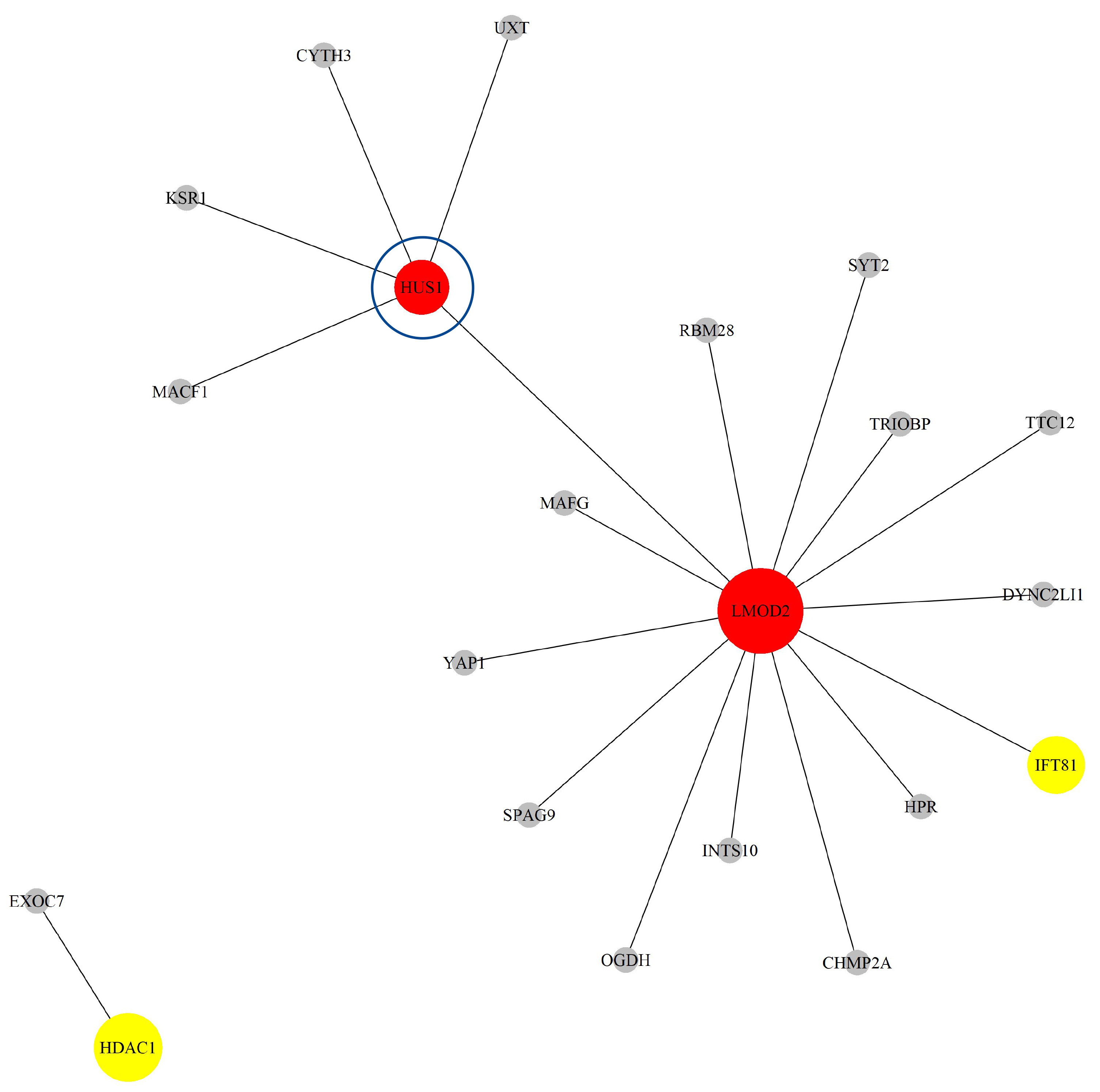
Next, based on the GO-CC pathway database, we apply our proposed method to the entire TCGA BLCA dataset for model selection and parameter estimation. The method identifies 23 genes and 19 gene-gene interaction biomarkers, with corresponding network structure shown in Fig. 9 with the top 10 highest and bottom 10 lowest biomarker coefficient values shown in Table 6. Supplementary Table 9 presents all the selected biomarkers and their corresponding coefficients.
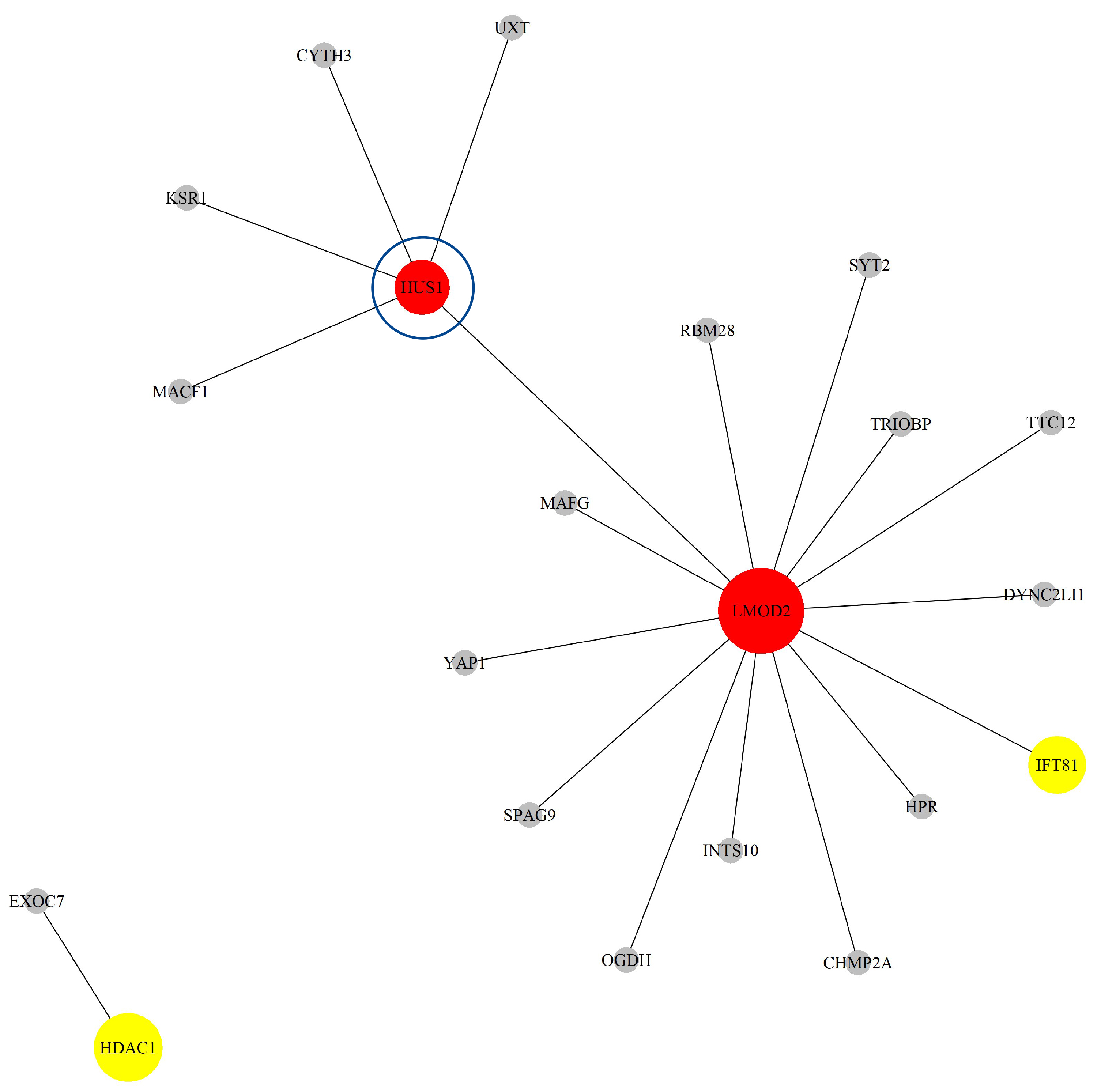 Fig. 9.
The Network structure of the selected G-G interaction by the proposed OGS_G.ridge_ALasso method in BLCA.
The HUS1 gene has been confirmed to have biological significance in the literature [43]. HUS1 is a protein involved in DNA repair, and its expression is elevated in BLCA. Studies indicate that inhibiting HUS1 enhances chemotherapy efficacy in cisplatin-sensitive cancer cells, but has no significant effect in resistant cells. Additionally, high expression of HUS1 is associated with poor prognosis in patients, suggesting that HUS1 might be a key factor influencing responses to platinum-based chemotherapy and could potentially serve as a therapeutic target.
Our TCGA LIHC dataset includes 334 subjects: 177 with BMI
We used a validation set approach, randomly splitting the dataset into 80% training (267 samples) and 20% testing (67 samples), and repeated this process 30 times after excluding 366 unmapped genes. Table 8 summarizes the average prediction results for BMI. We also evaluated two additional GO pathway databases: GO-BP and GO-MF with results in Supplementary Tables 10,11. Across all databases, OGS_G.ridge_ALasso outperformed other methods, including standard machine learning models, particularly in terms of SMAPE, while also showing strong results in other metrics.
| MinMax Accuracy | MAPE (%) | SMAPE (%) | RMSE | MASE | MAE | MDAE | |
| SIS_Lasso | –2.2580 (6.0536) | 332.4607 (207.7500) | 139.6710 (9.4129) | 1.0110 (0.4015) | 0.8912 (0.1631) | 0.6283 (0.0866) | 0.4656 (0.0606) |
| Ordinary_Lasso | –5.0734 (17.9602) | 308.1448 (220.9625) | 150.2410 (21.8989) | 0.9754 (0.4296) | 0.8445 (0.1218) | 0.5992 (0.0881) | 0.4467 (0.0603) |
| OGS_Ridge | 10.9704 (59.6618) | 330.3707 (252.2040) | 140.4011 (14.6550) | 1.0014 (0.3908) | 0.8703 (0.1600) | 0.6125 (0.0772) | 0.4506 (0.0534) |
| OGS_Lasso | 1.2601 (12.1217) | 385.5694 (322.1085) | 136.4481 (19.2138) | 1.0496 (0.3702) | 0.9144 (0.1894) | 0.6409 (0.0809) | 0.4601 (0.0770) |
| OGS_ALasso | –3.0848 (12.5386) | 453.0267 (331.5226) | 131.5387 (9.0808) | 1.0687 (0.3576) | 0.9497 (0.2076) | 0.6619 (0.0668) | 0.4751 (0.0544) |
| OGS_G.ridge | –7.7167 (27.3397) | 421.3698 (286.6483) | 131.7760 (8.6800) | 1.0424 (0.3687) | 0.9173 (0.1974) | 0.6414 (0.0751) | 0.4741 (0.0712) |
| OGS_G.ridge_ALasso | –2.0931 (5.4303) | 494.6527 (355.0585) | 132.5872 (9.1075) | 1.1132 (0.3379) | 1.0051 (0.2554) | 0.6951 (0.0692) | 0.5223 (0.0888) |
| OGS_SVR | –1.2808 (11.1659) | 270.0525 (202.1000) | 136.0872 (16.8650) | 0.9203 (0.4336) | 0.7729 (0.1013) | 0.5512 (0.0950) | 0.4034 (0.0674) |
| OGS_RF | 1.0304 (4.3231) | 300.3950 (188.4677) | 142.1591 (10.3168) | 1.1064 (0.4338) | 0.9349 (0.2765) | 0.6477 (0.1109) | 0.4667 (0.0652) |
| OGS_KNN | 0.9596 (6.5329) | 205.5634 (154.2807) | 156.1949 (18.8047) | 0.9444 (0.4359) | 0.8122 (0.1059) | 0.5771 (0.0845) | 0.4444 (0.0575) |
The table reports the mean (standard deviation) of the test prediction performance for various prediction methods.
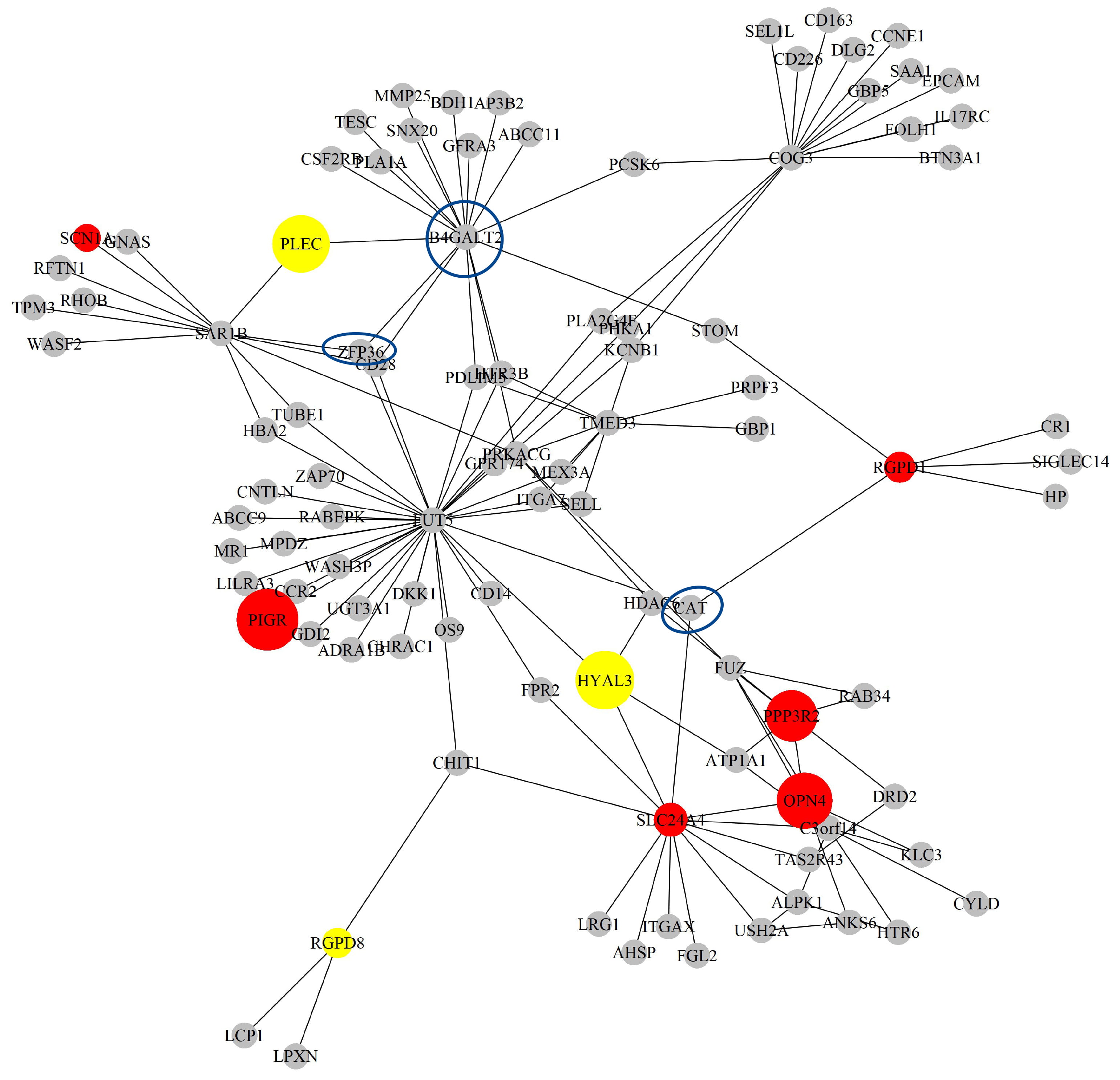
Next, based on the GO-CC pathway database, we apply our proposed method to the entire TCGA LIHC dataset for model selection and parameter estimation. The method identifies 16 genes and 132 gene-gene interaction biomarkers, with corresponding network structure shown in Fig. 10 with the top 10 highest and bottom 10 lowest biomarker coefficient values shown in Table 6. Supplementary Table 12 presents all the selected biomarkers and their corresponding coefficients.
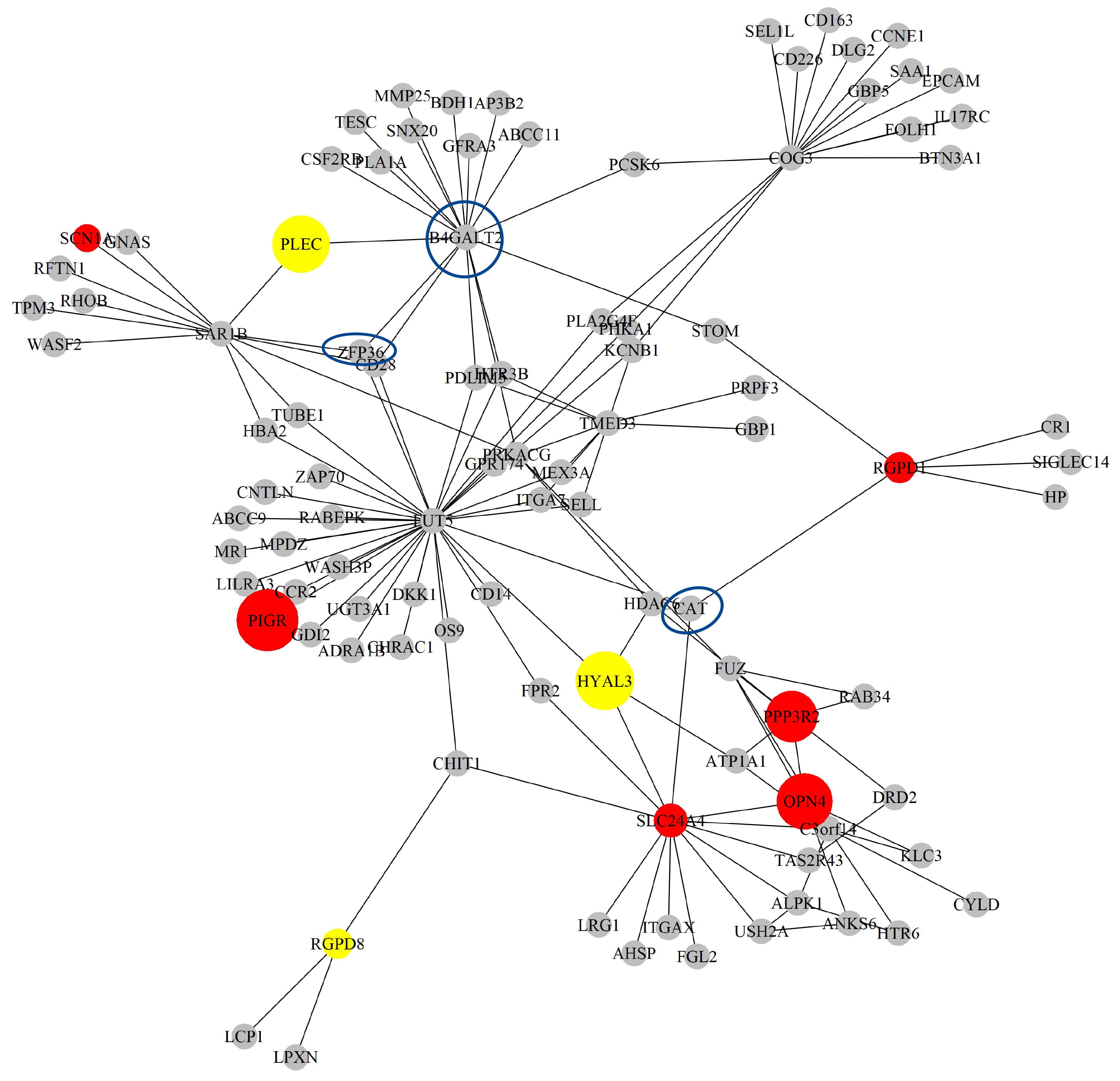 Fig. 10.
The Network structure of the selected G-G interaction by the proposed OGS_G.ridge_ALasso method in LIHC.
Among the selected biomarkers, some have already been confirmed in existing literature to hold biological significance. A study by Chen et al. [44] found that the expression of CAT was significantly downregulated in advanced LIHC tissues, and that high CAT expression was associated with better survival outcomes. Furthermore, when CAT expression is low, MET inhibitors such as SU11274 may serve as effective treatment options for LIHC with low CAT expression. This suggests that CAT might play an important role in LIHC and is closely related to tumor progression and prognosis. Wang et al. [45] reported that ZFP36 is a gene associated with ferritinophagy and exhibits abnormal expression in immune cells in LIHC with their results indicating that ZFP36 could be closely involved with the functions of monocytes and macrophages, and might participate in immune regulation and tumor progression. ZFP36 shows potential as a target for liver cancer research or therapy. Zhao et al. [46] identified B4GALT2 as a gene related to amino acid metabolism, which has been incorporated into a prognostic risk model for LIHC patients, and as its high expression is associated with poorer survival outcomes and could be involved in immune regulation and metabolic reprogramming in tumors, it has the potential to serve as a biomarker for liver cancer treatment and prognosis assessment.
Our TCGA ESCA dataset includes 175 subjects: 97 with BMI
We used a validation set approach, randomly splitting the dataset into 80% training (140 samples) and 20% testing (35 samples), and repeated this process 30 times after excluding 358 unmapped genes. Table 9 summarizes the average prediction results for BMI. We also evaluated two additional GO pathway databases: GO-BP and GO-MF with results in Supplementary Tables 13,14. Across all databases, Our proposed method (OGS_G.ridge_ALasso), while slightly outperformed by OGS_KNN in terms of the SMAPE (%) evaluation metric, still demonstrates better predictive performance compared to the other methods.
| MinMax Accuracy | MAPE (%) | SMAPE (%) | RMSE | MASE | MAE | MDAE | |
| SIS_Lasso | 2.7686 (4.0457) | 258.6933 (132.1144) | 108.7875 (11.2686) | 0.9117 (0.1998) | 0.7831 (0.1125) | 0.6334 (0.0923) | 0.4391 (0.0727) |
| Ordinary_Lasso | 1.7824 (6.6566) | 200.7705 (107.6323) | 114.7371 (12.8876) | 0.8606 (0.2394) | 0.7174 (0.0778) | 0.5876 (0.1151) | 0.4106 (0.0718) |
| OGS_Ridge | 1.1757 (1.5268) | 232.8646 (122.2114) | 105.6107 (14.1393) | 0.8431 (0.2280) | 0.7205 (0.1063) | 0.5881 (0.1141) | 0.4298 (0.0775) |
| OGS_Lasso | 0.9132 (1.7178) | 260.1778 (138.2418) | 107.1521 (15.4873) | 0.8670 (0.2226) | 0.7557 (0.1442) | 0.6135 (0.1221) | 0.4504 (0.0898) |
| OGS_ALasso | 1.4643 (4.8301) | 265.4442 (150.5444) | 107.4061 (15.3619) | 0.8640 (0.2260) | 0.7530 (0.1520) | 0.6111 (0.1248) | 0.4556 (0.1057) |
| OGS_G.ridge | –2.5742 (22.4868) | 237.4606 (127.2772) | 105.9300 (14.4189) | 0.8362 (0.2260) | 0.7178 (0.1154) | 0.5857 (0.1178) | 0.4391 (0.0878) |
| OGS_G.ridge_ALasso | 1.4586 (1.8296) | 257.2740 (140.6211) | 106.0141 (13.7132) | 0.8572 (0.2190) | 0.7408 (0.1260) | 0.6017 (0.1120) | 0.4454 (0.0850) |
| OGS_SVR | 2.0123 (2.7678) | 245.4466 (137.2884) | 109.6309 (12.6539) | 0.8647 (0.2128) | 0.7419 (0.1161) | 0.6021 (0.1052) | 0.4436 (0.0719) |
| OGS_RF | 1.4777 (6.2537) | 250.5895 (145.5156) | 106.9120 (11.5959) | 0.8387 (0.2223) | 0.7177 (0.1196) | 0.5836 (0.1064) | 0.4122 (0.0723) |
| OGS_KNN | 2.0430 (1.5909) | 246.6405 (134.6129) | 101.2479 (13.7206) | 0.8217 (0.2389) | 0.6823 (0.0743) | 0.5623 (0.1225) | 0.3886 (0.0786) |
The table reports the mean (standard deviation) of the test prediction performance for various prediction methods.
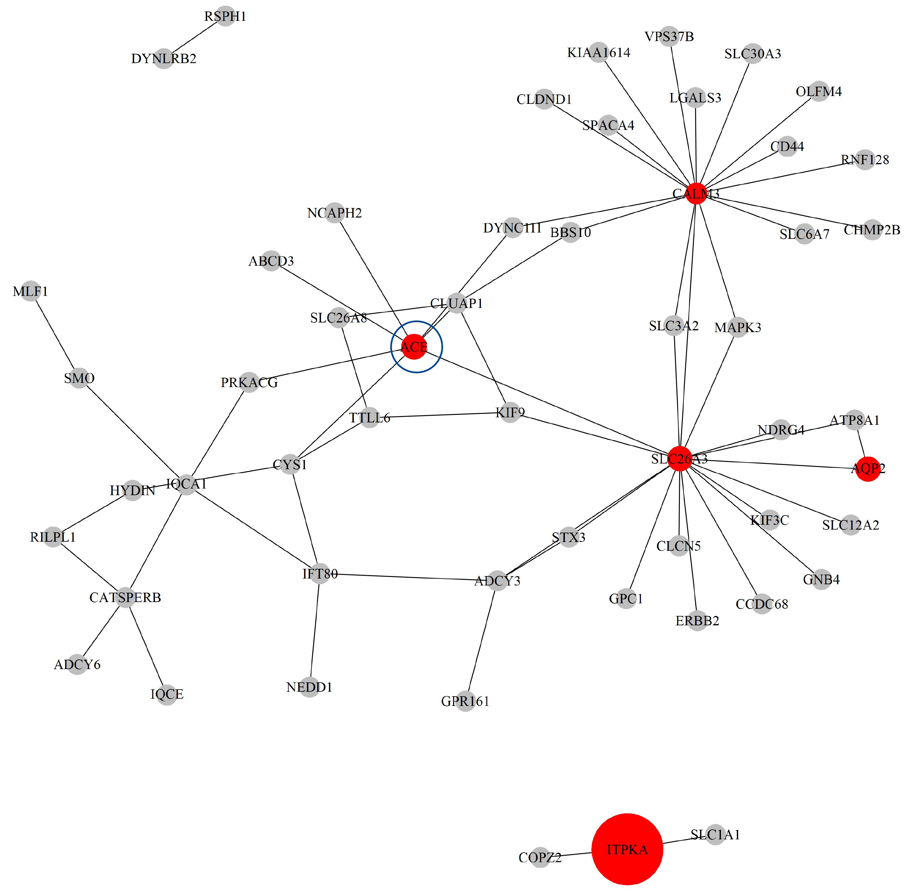
Next, based on the GO-CC pathway database, we apply our proposed method to the entire TCGA ESCA dataset for model selection and parameter estimation. The method identifies 8 genes and 63 gene-gene interaction biomarkers, with corresponding network structure shown in Fig. 11 with the top 10 highest and bottom 10 lowest biomarker coefficient values are shown in Table 6. Supplementary Table 15 presents all the selected biomarkers and their corresponding coefficients.
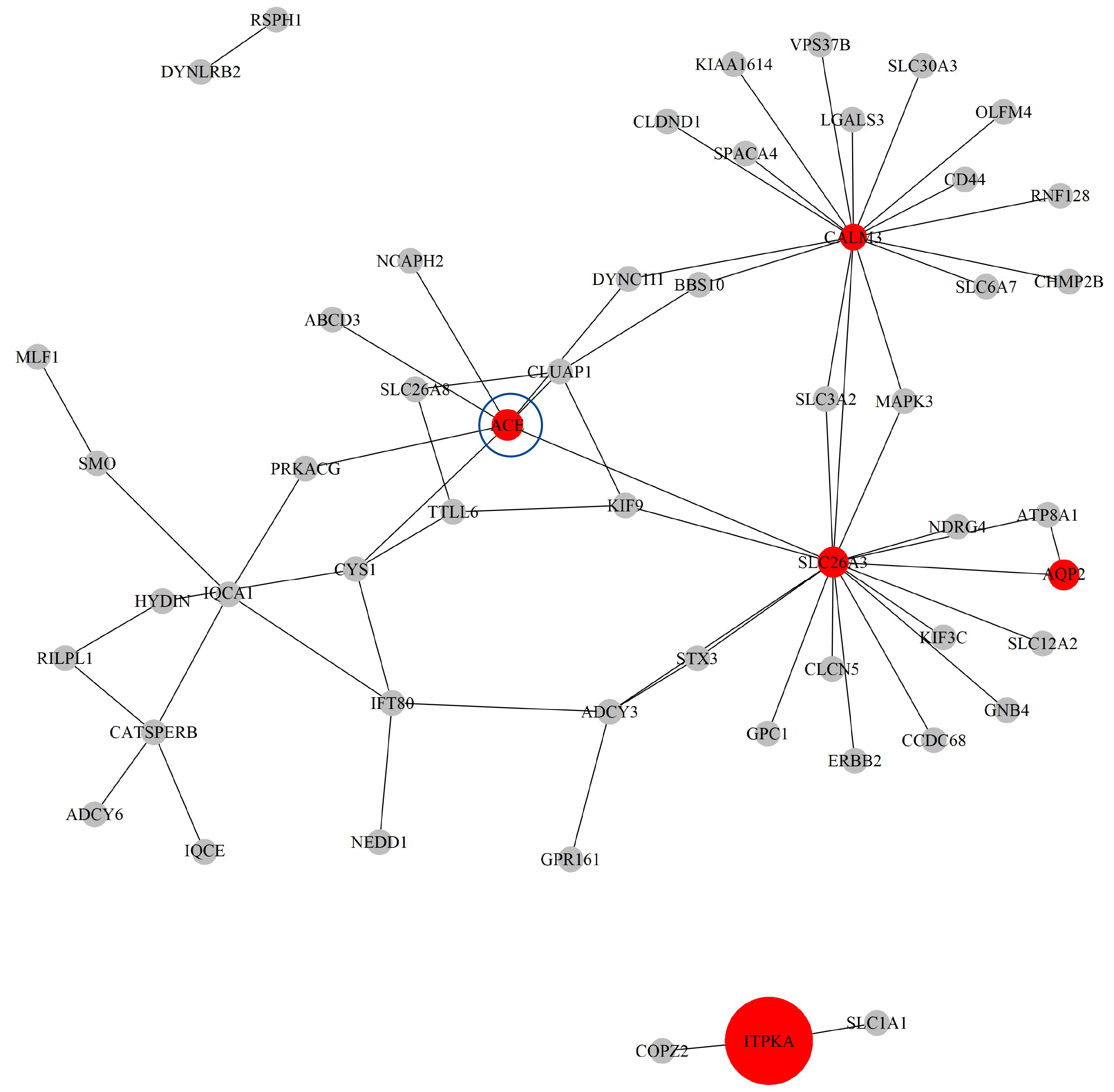 Fig. 11.
The Network structure of the selected G-G interaction by the proposed OGS_G.ridge_ALasso method in ESCA.
The ACE gene has been shown to have biological significance in the literature [47]. The study demonstrated that, among patients with esophageal cancer, those with the ACE gene D/D genotype were more likely to develop postoperative pulmonary complications, with a risk more than three times higher than that of patients with the I/I or I/D genotypes. In addition, serum ACE levels were positively correlated with the presence of the ACE D allele; the higher the ACE level, the greater the risk of postoperative pulmonary complications. This suggests that the insertion/deletion polymorphism of the ACE gene may could an important role in susceptibility to postoperative pulmonary injury in patients with esophageal cancer.
In this study, patients with various cancer types are stratified into three groups based on their BMI: normal, overweight and obese. Within each BMI subgroup, a Cox proportional hazards model is applied to assess the association between the expression level of individual genes and overall survival with each model including only one gene as the primary explanatory variable, and age and gender being incorporated as covariates to adjust for potential confounding effects. A stratified analytical approach is employed to evaluate whether BMI classification modulates the prognostic impact of gene expression on survival outcomes and to identify gene signatures with significant prognostic relevance within specific BMI categories. Gene selection is based on both the analytical framework developed in this study and relevant targets reported in the literature. The results are summarized in Table 10.
| Cancer Type | BMI Class | Number of Patients (events) | Coef (p-value) | Coef (p-value) | Coef (p-value) |
| CESC | WNT1 | CRK | |||
| Normal | 100 (26) | –0.2515 (0.340) | 0.2658 (0.248) | ||
| Overweight | 72 (10) | –0.4274 (0.4295) | 0.6888 (0.0611) | ||
| Obese | 86 (16) | –0.1744 (0.467) | 0.0592 (0.831) | ||
| BLCA | HUS1 | ||||
| Normal | 147 (54) | –0.0550 (0.6725) | |||
| Overweight | 124 (62) | 0.1361 (0.3170) | |||
| Obese | 85 (34) | –0.0227 (0.8864) | |||
| LIHC | CAT | ZFP36 | B4GALT2 | ||
| Normal | 177 (61) | –0.2142 (0.0578) | 0.0341 (0.769) | 0.2113 (0.0979) | |
| Overweight | 89 (28) | –0.7447 (0.0005) | 0.0217 (0.931) | 0.4846 (0.0227) | |
| Obese | 68 (23) | –0.0227 (0.9282) | –0.3233 (0.1300) | 0.0242 (0.9189) | |
| ESCA | ACE | ||||
| Normal | 97 (35) | 0.0074 (0.969) | |||
| Overweight | 49 (19) | –0.2145 (0.3558) | |||
| Obese | 29 (16) | 0.1242 (0.630) |
The results show that most genes do not exhibit statistically significant associations with overall survival across different cancer types and BMI subgroups. However, in LIHC, the expression of the CAT gene in the overweight group is significantly negatively associated with overall survival (coefficient = –0.7447, p = 0.0005), indicating a potential protective prognostic role. In contrast, the B4GALT2 gene shows a significant positive association (coefficient = 0.4846, p = 0.0227), suggesting it might function as a risk factor. Additionally, in CESC, the expression of the CRK gene in the overweight group demonstrates a borderline significant positive association (p = 0.0611). Overall, the findings indicate that specific genes are significantly associated with survival only within certain BMI categories, suggesting that BMI could act as a modifier of gene-based prognostic effects and warrants further investigation into the underlying biological mechanisms.
We perform Kaplan-Meier survival analyses within each BMI subgroup, using the median gene expression as a cutoff. Several genes show significant or borderline associations with overall survival in specific BMI categories (Supplementary Figs. 1–7). WNT1 is significantly associated with survival in the normal BMI group (p = 0.0036), while CAT shows protective associations in both the normal (p = 0.0028) and overweight (p = 0.0087) groups. B4GALT2 is linked to worse survival in the normal group (p = 0.037), and CRK shows a borderline association in the overweight group (p = 0.059). HUS1 (p = 0.1) and ZFP36 (p = 0.1) also display borderline significance in the normal and obese groups. These results suggest that BMI could modify the prognostic impact of gene expression.
To better interpret the biological significance of gene expression data, we analyzed not only individual genes but also gene sets with functional or regulatory relevance. Model-based Gene Set Analysis (MGSA) is a Bayesian approach that reveals expression patterns and functional relationships among gene sets within biological systems [48]. MGSA integrates pathway information and statistical modeling to evaluate gene set changes under different conditions, helping to understand their impact on diseases or physiological states. This method is implemented in the R package “mgsa” and incorporates Gene Ontology data [49]. In this study, we identified important genes using our proposed method, OGS_G.ridge_ALasso, and annotate them based on gene sets from the MSigDB database, including collections such as c2.cp.biocarta, c2.cp.kegg, c5.GOBP, c5.GOCC and c5.GOMF.
Using MGSA, we identified multiple biologically relevant pathways significantly associated with BMI across different cancers. In BLCA, GOBP_INTRACILIARY_TRANSPORT_INVOLVED_IN_CILIUM_ASSEMBLY, related to cilium assembly and intraciliary transport, links to BMI, highlighting processes crucial for cell polarity and signal transduction. In ESCA, KEGG_MEDICUS_REFERENCE_AVP_V2R_PKA_SIGNALING_PATHWAY, involving antidiuretic hormone signaling via the V2 receptor and PKA activation, associates with BMI, implicating metabolism and intracellular signaling regulation. In CESC, GOBP_REGULATION_OF_NEUROMUSCULAR_JUNCTION_DEVELOPMENT, which regulates neuromuscular junction formation and function, correlates with BMI. Finally, in LIHC, GOBP_NEGATIVE_REGULATION_OF_HYDROGEN_PEROXIDE_METABOLIC_PROCESS, involved in negative regulation of hydrogen peroxide metabolism and oxidative stress response, shows significant association with BMI. These findings support the biological relevance of the identified biomarkers and provide insight into the pathways through which BMI may influence cancer biology.
Identifying susceptibility genes and variants for complex diseases is challenging due to the often unknown underlying disease mechanisms. The OGS method, which incorporates the SKAT to screen for gene-gene interactions, relies on predefined pathways to extract gene network information although such reliance might lead to information loss while limiting the method’s scope; additionally, while current implementations typically consider only simple two-way or multiplicative interactions, future research should aim to develop statistical approaches capable of capturing higher-order and more complex interactions.
Multivariate analysis is another widely used approach, testing grouped variants defined by genes, pathways, or physical locations. Common statistical methods include burden tests, SKAT and the combined SKAT-O, each showing strengths under different biological conditions [50] Data-adaptive methods, which adjust models based on the data structure, have attracted increasing attention. Notably, Ueki [51] proposed a novel approach based on Yanai’s generalized coefficient of determination, which allows for the control of type I error without requiring test-specific null distributions. This method is computationally efficient and broadly applicable to models such as lasso, ridge and elastic net, enabling both variant selection and feature filtering. In summary, future efforts should focus on developing more flexible, accurate and interpretable methods to improve the detection of relevant variants in genome-wide studies.
TCGA provides a rich and comprehensive resource for exploring the relationship between BMI and cancer. With its extensive genomic and clinical datasets spanning numerous cancer types, TCGA enables multi-omics analyses—integrating gene expression, somatic mutations, DNA methylation and copy number variations. This multi-layered approach allows for a deeper understanding of how BMI could influence cancer biology at the molecular level [52], while its pan-cancer structure facilitates cross-tumor comparisons, helping to uncover both shared and cancer-specific BMI-related molecular features.
We agree that validating BMI-associated gene signatures in independent cohorts is a crucial step to enhance the generalizability of our findings. We have reviewed multiple external datasets from sources such as Gene Expression Omnibus (GEO) and International Cancer Genome Consortium (ICGC) and confirmed that some do include BMI-related annotations [53, 54]. Although external validation was not performed in the current study, we fully recognize its importance in establishing the broader applicability of our results. Future studies should consider validating the gene signatures identified here using independent datasets with BMI information, although owing to considerable heterogeneity in data generation platforms and clinical variable definitions, incorporating such datasets would require extensive data harmonization and standardization efforts, introducing complexity beyond the scope of this study. In light of these challenges, we focused on leveraging the pan-cancer framework of TCGA to assess the internal consistency and robustness of BMI-associated gene signatures across multiple cancer types. These results provide preliminary support for the validity of our findings.
In our current simulated and real data analysis, BMI was treated as a continuous variable rather than categorized into discrete groups. This modeling approach allowed us to avoid arbitrary threshold effects and better capture dose-dependent associations between BMI and clinical or molecular outcomes. As such, the issue of cutoff definition (e.g., WHO vs. Asian-specific thresholds) did not directly affect our core statistical framework; nonetheless, we fully acknowledge the importance of population-specific BMI classification when translating findings into clinical practice.
The widely used BMI classification system—defining 18.5–24.9 as normal, 25+ as overweight and 30+ as obese—is based predominantly on data from Western populations, although research on individuals of Asian descent often exhibit higher body fat percentages at the same BMI levels along with increased susceptibility to chronic conditions such as cancer, type 2 diabetes, hypertension and cardiovascular disease. Consequently, applying Western BMI thresholds to Asian populations might lead to underestimation of health risks.
To address this disparity, region-specific resources such as the Taiwan Biobank and Taiwan’s National Health Insurance Research Database offer valuable Asian population-based insights. These have informed proposals to lower the overweight and obesity thresholds to 23 and 27 for Asian populations respectively, in the endeavor to enhance disease risk prediction and improve public health strategies. Looking ahead, the integration of genetic, dietary and environmental factors holds promise for advancing more personalized and accurate health assessment models.
Although this study utilizes TCGA data to investigate the relationship between obesity and cancer prognosis and observes the so-called “obesity paradox” in certain contexts, where patients with higher BMI exhibit better outcomes, these findings should be interpreted with caution. The TCGA dataset lacks many potential confounding variables such as treatment history, comorbidities (e.g., diabetes) and lifestyle factors (e.g., smoking and physical activity), which might lead to residual confounding and distort the true relationship between obesity and prognosis. Furthermore, BMI is measured at a single time point, limiting the ability to capture weight changes over time and to differentiate between fat and muscle mass. The retrospective nature of the study design further constrains causal inference; accordingly, future prospective cohort studies with more comprehensive clinical data are warranted to clarify the true causal relationship between obesity and cancer prognosis and validate the observed “obesity paradox” phenomenon reported in this study.
Regarding experimental validation such as qPCR or Western blot, we agree that such assays could further strengthen the biological significance of our findings. However, these experiments fall beyond the current scope and resources of this study, which is primarily computational in nature. Although this study does not include laboratory-based experimental validation, we conducted pathway enrichment analysis using the MGSA method to explore the functional relevance of the top-ranked BMI-associated genes, with results indicating that these genes could be involved in metabolic and inflammatory pathways known to be associated with obesity and cancer progression.
This study focuses on four cancer types: BLCA, CESC, LIHC and ESCA, selected based on their sample sizes, BMI distributions and biological characteristics. However, the current results are not yet placed within the broader TCGA pan-cancer framework, which might limit the generalizability of the findings. Notably, LIHC and ESCA show lower obesity rates, which likely relate to their unique disease etiologies and risk factors such as viral infections, alcohol consumption or chronic hepatitis thereby possibly weakening the association between BMI and cancer outcomes; additionally, the interactions between BMI and gene expression vary across cancer types, suggesting that the prognostic impact of BMI could be cancer-type specific. Future research should expand analysis to additional cancer types to more comprehensively assess the universality and biological relevance of BMI-associated gene signatures.
This study highlights the critical role of BMI in cancer development and prognosis, using TCGA data for in-depth analysis. Both high and low BMI levels were found to be linked to increased cancer risk, where obesity plays a role through hormonal imbalance, inflammation and immune dysfunction, while at the same time, underweight individuals might suffer from malnutrition and reduced treatment tolerance. BMI also affects treatment outcomes: obese patients often face higher complication risks, while underweight individuals might recover less effectively. Interestingly, the “obesity paradox” suggests that in some cancers, higher BMI can be linked to better survival, underscoring the complex, context-dependent nature of the BMI–cancer relationship.
Using the OGS method combined with regularized regression, particularly the OGS_G.ridge_ALasso model, we identified BMI-related genes and interactions from high-dimensional genetic data. This model performed best in accuracy and consistency, particularly in settings with overlapping genetic signals. By applying it to TCGA data, we uncovered meaningful molecular links between BMI and cancer, supporting the importance of maintaining a healthy BMI and offering a framework for exploring gene networks and biomarkers that can inform personalized cancer care.
ABC, Advanced breast cancer; ALasso, Adaptive lasso; BLCA, Bladder urothelial carcinoma; BMI, Body mass index; BP, Biological process; CC, Cellular composition; CESC, Cervical squamous cell carcinoma and endocervical adenocarcinoma; COAD, Colon adenocarcinoma; COADREAD, Colorectal adenocarcinoma; DNA, eoxyribonucleic acid; EBC, Early breast cancer; ESCA, Esophageal carcinoma; GEO, Gene Expression Omnibus; G-G, gene-gene interaction; GO, Gene ontology; G.ridge, Generalized ridge regression; ICGC, International Cancer Genome Consortium; IQR, Interquartile range; KIRP, Kidney renal papillary cell carcinoma; KNN, k-nearest neighbors; lasso, Least absolute shrinkage and selection operator; LIHC, Liver hepatocellular carcinoma; MAE, Mean absolute error; MDAE, Median absolute error; MAPE, Mean absolute percentage error; MASE, Mean absolute scaled error; MCP, Minimax concave penalty; MF, Molecular function; MGSA, Model-based Gene Set Analysis; ML, Machine learning; MSigDB, The human molecular signature database; NSCLC, Non-small cell lung cancer; OGS, Overlapping group screening; OLS, Ordinary least squares regression; RF, Random forest; RMSE, Root mean squared error; SMAPE, Symmetric mean absolute percentage error; SCAD, Smoothly clipped absolute deviation; SIS, Sure independence screening; SKAT, Sequence kernel association test; SVR, Support vector regression; TCGA, The Cancer Genome Atlas; UCSC, University of California, Santa Cruz; WHO, World health organization.
The TCGA transcriptomic data for CESC, BLCA, LIHC and ESCA, along with the clinical BMI outcomes analyzed in this study and the R scripts used for both simulation and real data analyses are available from the corresponding author upon reasonable request. The TCGA data were originally obtained from the TCGA Hub repository (https://tcga.xenahubs.net), with the primary source being the TCGA website (https://www.cancer.gov/ccg/research/genome-sequencing/tcga).
JHW conceived and designed the experiments. JHW, ZHW and TCC collected and organized the analysis data. JHW and HCL analyzed the data. JHW wrote the first draft of the manuscript. JHW made critical revisions and approved final version. All authors agreed with manuscript results and conclusions. All authors jointly developed the structure and arguments for the paper. All authors reviewed and approved of the final manuscript. All authors contributed to editorial changes in the manuscript. All authors have participated sufficiently in the work and agreed to be accountable for all aspects of the work.
Not applicable.
The authors sincerely thank Mr. Tzung-Ying Guo and Mr. Po-Lin Hou from the Department of Mathematics, National Chung Cheng University, for their invaluable assistance in creating figures, organizing tables, and assisting with the implementation of the MGSA method during the revision of this article. The results shown here are in whole or part based upon data generated by the TCGA Research Network: https://www.cancer.gov/tcga.
This research was supported by the grant NSTC 112-2118-M-194-003-MY2 from the National Science and Technology Council of Republic of China (Taiwan). The funding body did not play any role in the design of the study and collection, analysis, and interpretation of data and in writing the manuscript.
The authors declare no conflict of interest.
During the preparation of this work, the authors used ChatGPT solely for spelling and grammar checking in the manuscript writing stage. The selection of the research topic, design of statistical methods, programming, simulations and data analysis were independently conducted by the authors and are entirely original. After using the AI tool, the authors carefully reviewed its suggestions and made revisions as needed, taking full responsibility for the final submitted content.
Supplementary material associated with this article can be found, in the online version, at https://doi.org/10.31083/FBL43294.
References
Publisher’s Note: IMR Press stays neutral with regard to jurisdictional claims in published maps and institutional affiliations.