


 , Yuan Chen 1,*
1 Hunan Engineering & Technology Research Centre for Agricultural Big Data Analysis & Decision-Making, Hunan Agricultural University, 410128 Changsha, Hunan, China
Abstract
Background: Ubiquitination is a crucial post-translational modification of proteins that regulates diverse cellular functions. Accurate identification of ubiquitination sites in proteins is vital for understanding fundamental biological mechanisms, such as cell cycle and DNA repair. Conventional experimental approaches are resource-intensive, whereas machine learning offers a cost-effective means of accurately identifying ubiquitination sites. The prediction of ubiquitination sites is species-specific, with many existing models being tailored for Arabidopsis thaliana (A. thaliana) and Homo sapiens (H. sapiens). However, these models have shortcomings in sequence window selection and feature extraction, leading to suboptimal performance. Methods: This study initially employed the chi-square test to determine the optimal sequence window. Subsequently, a combination of six features was assessed: Binary Encoding (BE), Composition of K-Spaced Amino Acid Pair (CKSAAP), Enhanced Amino Acid Composition (EAAC), Position Weight Matrix (PWM), 531 Properties of Amino Acids (AA531), and Position-Specific Scoring Matrix (PSSM). Comparative evaluation involved three feature selection methods: Minimum Redundancy-Maximum Relevance (mRMR), Elastic net, and Null importances. Alongside these were four classifiers: Support Vector Machine (SVM), Decision Tree (DT), Random Forest (RF), and Extreme Gradient Boosting (XGBoost). The Null importances combined with the RF model exhibited superior predictive performance, and was denoted as UbNiRF (A. thaliana: ArUbNiRF; H. sapiens: HoUbNiRF). Results: A comprehensive assessment indicated that UbNiRF is superior to existing prediction tools across five performance metrics. It notably excelled in the Matthews Correlation Coefficient (MCC), with values of 0.827 for the A. thaliana dataset and 0.781 for the H. sapiens dataset. Feature analysis underscores the significance of integrating six features and demonstrates their critical role in enhancing model performance. Conclusions: UbNiRF is a valuable predictive tool for identifying ubiquitination sites in both A. thaliana and H. sapiens. Its robust performance and species-specific discovery capabilities make it extremely useful for elucidating biological processes and disease mechanisms associated with ubiquitination.
Keywords
- ubiquitination site
- chi-square test
- null importances
- random forest
Ubiquitin is a small protein comprised of 76 amino acid residues. This protein is strongly conserved across eukaryotic cells. Ubiquitination is the post-translational process whereby ubiquitin molecules attach to lysine residues on substrate proteins. This process regulates various cellular functions including cell cycle progression, DNA repair, transcriptional control, receptor trafficking, immune response, viral infection, etc. [1, 2, 3]. Dysregulation of ubiquitination in humans can result in cancer and neurodegenerative diseases [4, 5, 6], while in plants it can impact growth, development, and responses to biotic and abiotic stresses [7, 8]. Accurate identification of protein ubiquitination sites is crucial for understanding cellular functions and network regulation. Traditional methods for detecting ubiquitination sites, such as Chromatin Immunoprecipitation (ChIP) [9], Mass Spectrometry (MS) [10], and liquid chromatography [11], are laborious, time-consuming, and costly. However, rapid advances in machine learning technology may offer a cost-effective and accurate way to identify ubiquitination sites.
Ubiquitination sites exhibit significant species specificity, with the current machine learning-based prediction methods primarily targeting Arabidopsis thaliana (A. thaliana) and Homo sapiens (H. sapiens). The prediction process for ubiquitination modification sites typically encompasses five essential stages: window size determination, feature extraction, feature selection, classifier choice, and performance evaluation.
(1) Window size determination. Selection of an optimal window size is crucial for accurate prediction of ubiquitination sites. Current reports encompass ranges such as –10~+10 [12], –13~+13 [13, 14, 15, 16], –20~+20 [17, 18, 19], all of which are centered around lysine ‘K’. However, there is no clear rationale guiding the selection.
(2) Feature extraction. Feature extraction involves deriving the predictive attributes from protein sequences and converting string sequences into digital formats. Widely employed methods for feature extraction in site prediction encompass Binary Encoding (BE) [18], Composition of K-Spaced Amino Acid Pair (CKSAAP) [20, 21], Position Weight Matrix (PWM) [22], Amino Acid Composition (AAC) [17], Enhanced Amino Acid Composition (EAAC) [19, 23, 24], 531 Properties of Amino Acids (AA531) [12], Position-Specific Scoring Matrix (PSSM) [25, 26], Blocks Substitution Matrix (BLOSUM62) [19], etc. The majority of models tend to incorporate only one feature, or 2–3 features, and lack the integration of multiple feature types.
(3) Feature selection. Feature selection is a crucial aspect of machine learning, with profound impacts on model accuracy, reduction of runtime, and enhancement of interpretability. Common feature selection methodologies employed in bioinformatics include Minimum Redundancy-Maximum Relevance (mRMR) [27], Elastic net [28], and Null importances [29].
(4) Classifier choice. During model construction, multiple classifiers for comparative analysis and selection are commonly used to enhance prediction accuracy and stability. Each classifier has distinct strengths and weaknesses, and caters to diverse datasets or specific contexts. Notable predictors include Support Vector Machine (SVM) [30], Decision Tree (DT) [31], Random Forest (RF) [32], and Extreme Gradient Boosting (XGBoost) [33].
(5) Performance evaluation. Cross-validation and independent testing are commonly used to evaluate model performance. Cross-validation is used primarily to assess the model’s generalization on training data. Post cross-validation, further testing on a separate, unused dataset is crucial to ascertain true model performance. For the A. thaliana model, the cross-validated Matthews Correlation Coefficient (MCC) ranges from 0.485 to 0.822, with the Area Under the Receiver Operating Characteristic Curve (ROC curve, AUC) ranging from 0.877 to 0.977. Moreover, independently tested MCC ranges from 0.468 to 0.772, with an AUC range of 0.868 to 0.960 [16, 17, 18, 19]. For the H. sapiens model, the cross-validated MCC is 0.530 with an AUC range of 0.770 to 0.852, while the independent test MCC ranges from 0.480 to 0.673 and the AUC ranges from 0.757 to 0.950 [12, 13, 14, 15]. The existing models indicate there is still a need to improve both MCC and AUC, with a particular focus on enhancing MCC.
This study addresses several of the above key aspects. Firstly, the chi-square test was employed to determine the optimal size of the protein sequence window within the dataset. Subsequently, a fusion feature set incorporating six distinct features (BE, PWM, CKSAAP, EAAC, AA531, and PSSM) was extracted. Three distinct feature selection methods (mRMR, Elastic net, and Null importances) were compared, alongside the evaluation of four classifiers (SVM, DT, RF, and XGBoost). To mitigate the imbalance between positive and negative samples, the Synthetic Minority Over-sampling Technique (SMOTE) was also introduced during the training phase [34], coupled with the application of stratified sampling in cross-validation. Following rigorous experimental comparisons, a combination of the null importances feature selection method and the RF classifier were found to show superior performance. Consequently, the UbNiRF model (A. thaliana: ArUbNiRF; H. sapiens: HoUbNiRF) was formulated. This showed several notable improvements compared to existing models. Furthermore, species-specificity for the prediction of ubiquitination sites was confirmed through species cross-testing of the ArUbNiRF model for A. thaliana and the HoUbNiRF model for H. sapiens. This demonstrated distinct predictive capabilities for different species. Additionally, we investigated the necessity to fuse the six features. The flowchart for the development of UbNiRF is shown in Fig. 1.
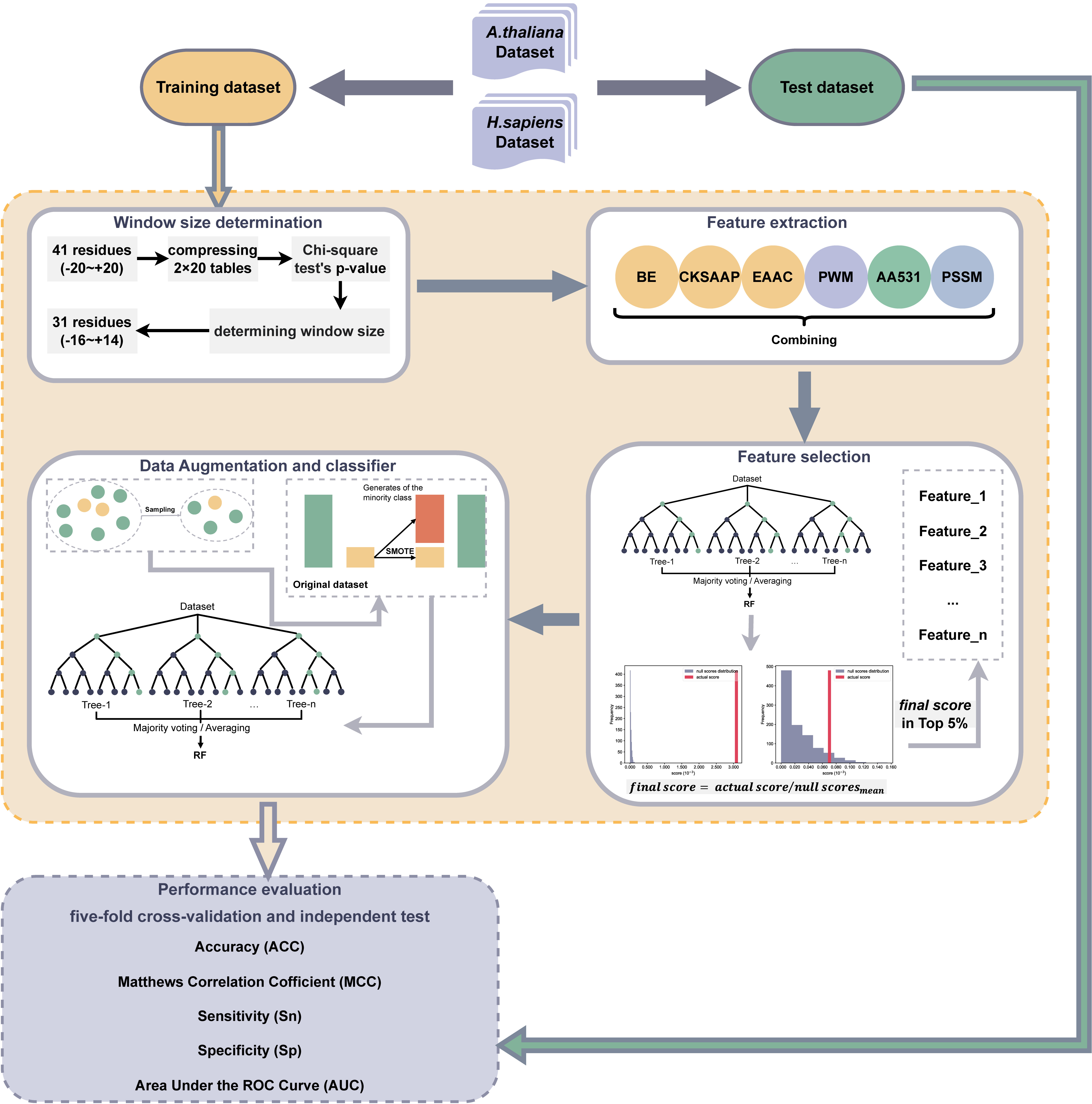 Fig. 1.
Flowchart for the development of UbNiRF. BE, Binary Encoding; CKSAAP, Composition of K-Spaced Amino Acid Pair; EAAC, Enhanced Amino Acid Composition; PWM, Position Weight Matrix; AA531, 531 Properties of Amino Acids; PSSM, Position-Specific Scoring Matrix.
To train and evaluate the proposed method, this study employed two ubiquitination site datasets from AraUbiSite (A. thaliana) [17] and HUbipPred (H. sapiens) [15]. Experimentally confirmed ubiquitination sites in these datasets are marked as positive samples, while the remaining lysine (‘K’) residues serve as negative samples (non-ubiquitination sites). Samples consist of A. thaliana sequence fragments with a window size of 41 and centered on lysine (‘K’). If the site is at the start or end of the sequence, thereby creating a peptide shorter than 41, ‘X’ fills the start or end of the peptide. In contrast, the H. sapiens dataset employs a window size of 27. CD-HIT software (canva.com.) [35] with a threshold of 40% sequence identity was applied to the A. thaliana dataset to remove redundant fragments in the compiled sequence fragments of positive and negative samples. The H. sapiens dataset utilizes the Blastclust program with a 30% identity cutoff for the same purpose, but with a notable window length of 27. Consequently, the current study reacquired the protein sequences via ID mapping (date: 2023-10-13) from the Uniprot database [36] in order to adjust the window length to 41. During ID mapping, some protein sequences were found to be missing from the Uniprot database, leading to fewer samples in the H. sapiens dataset compared to the original. Details of the A. thaliana and H. sapiens training and test datasets used in the model construction are presented in Table 1 (Ref. [15, 17]).
A chi-square independence test was performed to analyze the amino acid
distribution at each position in the A. thaliana and H. sapiens
training sets, excluding position 0. If the association between the sample label
and the amino acid distribution is statistically significant (p-value
 Fig. 2.
–lg(p-value) for different positions in the training datasets of A. thaliana and H. sapiens. (A) –lg(p-value) for different positions in the training dataset of A. thaliana. (B) –lg(p-value) for different positions in the training dataset of H. sapiens.
We next reviewed the established methodologies and utilized six prevalent and efficient numerical feature extraction methods for sequences. These included: (1) sequence composition information encompassing BE, CKSAAP, and EAAC; (2) positional information denoted by PWM; (3) physical and chemical property information referred to as AA531; and (4) evolutionary information represented by PSSM. Subsequently, these six features, amounting to a collective dimensionality of 20272, were fused for feature selection.
BE [38] is employed for feature extraction based on sequence composition
information. It is utilized to transform protein sequences into digital vectors.
With this approach, each amino acid is depicted as a 20-dimensional binary
vector. For instance, alanine (‘A’) is denoted as
[1,0,0,0,0,0,0,0,0,0,0,0,0,0,0,0,0,0,0,0], and arginine (‘R’) by
[0,1,0,0,0,0,0,0,0,0,0,0,0,0,0,0,0,0,0,0]. The special character ‘X’ is
distinguished as a 20-dimensional vector consisting of zeros:
[0,0,0,0,0,0,0,0,0,0,0,0,0,0,0,0,0,0,0,0]. Consequently, a protein sequence of
length L generates a feature vector with dimensions of 20
CKSAAP [39] is a feature extraction method that relies on protein sequence
composition and emphasizes the occurrence frequency of distinct pairs of amino
acids within amino acid fragments (total of 20
EAAC utilizes sequence composition to capture the frequency of standard amino
acid occurrences within individual peptide sequences. AAC transforms the 20 amino
acids into a 20-dimensional digital vector by tallying the occurrence of specific
amino acids in individual peptide sequences [40]. EAAC differs significantly from
this by employing continuous sliding from the N-terminus to the C-terminus of
peptide sequences, utilizing a fixed-length sliding window for computation [41].
Thus, for a protein sequence of length L, a fixed sliding window size of 5 would
yield L-5+1 sliding windows. The EAAC encoding dimension is (L-5+1)
PWM [22] represents a positional feature extraction method. For both positive and negative samples, the respective relative frequencies of the 20 amino acids at specific positions are calculated, thus giving the frequency data for amino acids at each position. Hence, a protein sequence of length L yields an L-dimensional feature vector.
The Amino Acid Index (AAindex) compiles numerical indices encompassing diverse
physicochemical and biochemical attributes of amino acids and their pairs [42]. A
total of 531 prevalent physical and chemical properties were employed for feature
extraction in this study. For each property, the average of the 20 amino acids
was computed for the placeholder character ‘X’. For a protein sequence of length
L, 531 physical and chemical properties were extracted per amino acid, resulting
in a feature matrix with dimensions of 531
PSSM is a method for extracting features rooted in evolutionary information. Position Specific Iterative-Blast (PSI-BLAST) is widely employed for identifying remotely-related protein sequences. PSSM generation involves comparing the target sequence against homologous sequences through PSI-BLAST as follows [43]:
The protein sequence P, of length L, can be transformed into a feature matrix
denoted as PSSMp, with the dimensions of L
Following the fusion of six features, the potential increase in feature dimensions might adversely impact both computational speed and model performance. Consequently, this study compared three feature selection methods: Null importances, mRMR, and Elastic net.
The Null importances method [29] is a statistical approach used to assess the significance of feature importance generated by the RF model. It involves creating a distribution of importance scores for each feature under the null hypothesis, which assumes that the feature is irrelevant to the prediction outcome. The process is carried out by permuting the response vector in the dataset and then re-running the model to compute importance scores for each feature. These permutations effectively break any real association between the feature and the target, thereby providing a baseline distribution of importance scores under the assumption of no relationship.
Integration of the null importances method with the RF model allows for a more robust assessment of feature importance. After the RF model is fitted on the original dataset, the original importance score of each feature is calculated. The null importances distribution is then generated by repeatedly permuting the response vector and recalculating each feature’s importance score across multiple iterations. The original importance scores can then be compared against this null distribution to determine the significance of the observed importances. Features with the original importance score significantly higher than those observed in the null distribution are considered to be genuinely informative for the model’s predictions, thereby providing a means to identify and focus on the most relevant features for the problem at hand.
This method enhances the interpretability of the RF model by distinguishing between features that have a statistically significant impact on the model’s predictions and those that do not. It also reduces the risk of over-interpreting importance scores derived from random noise in the data, thereby resulting in more reliable and transparent machine learning models.
Olivier implemented this method within the Kaggle Community (https://www.kaggle.com/code/ogrellier/feature-selection-with-null-importances). Drawing inspiration from this method, we implemented the following steps for feature selection: (1) Eliminate features exhibiting zero variance; (2) Employ random forest (default parameters) to compute the score for each feature within the original dataset (recorded as the actual score); (3) Randomly shuffle labels and employ random forest (default parameters) to derive scores for each feature. The resulting scores after label shuffling denote the null score for each feature. This process is repeated 1000 times to obtain the score distribution, and recorded as null scores for subsequent use. The custom scoring function is defined as follows:
The final score for each feature is computed using formula (2), features with a final score of 0 are eliminated, and the top 5% of features are selected as the ultimate input variables.
The mRMR algorithm is predicated on the principle of maximizing the relevance of selected features with respect to the target variable, while concurrently minimizing the redundancy among these features. The dual objectives of the mRMR algorithm ensure that the selected feature subset has a high degree of predictive power for the target variable, and is devoid of superfluous or duplicative information that could impair model performance. The mRMR algorithm operates by iteratively evaluating the mutual information between each feature and the target variable, thereby quantifying the relevance of each feature. Simultaneously, it assesses the mutual information among the features themselves to gauge their redundancy. The algorithm seeks to construct a feature subset where the average mutual information between the features and the target is maximized, and the average mutual information among the features is minimized. This approach facilitates the selection of a feature set that is both highly informative and minimally redundant, thus striking a balance between relevance and redundancy [27]. To implement the mRMR algorithm, we utilized the mrmr_classif function available in the mrmr package (version: 0.2.8) for Python (https://github.com/smazzanti/mrmr). The parameter K was set to match the number of features selected by the Null importances method, while retaining default values for the remaining parameters.
Elastic net is a regularization method that integrates the strengths of both the Ridge (L2 norm) and Lasso (L1 norm) regularization techniques. This integration is achieved by combining their penalty terms into a single formulation, thereby enabling the method to acquire the benefits of both approaches: Lasso’s capability for feature selection through its tendency to produce coefficients that are exactly zero, and Ridge’s ability to handle multicollinearity by more evenly distributing the penalty across all coefficients [44]. The sklearn.linear_model.ElasticNet class (https://scikit-learn.org/stable/modules/generated/sklearn.linear_model.ElasticNet.html) within the sklearn library was utilized to implement Elastic net for feature selection under the default parameter settings. These default parameters, including the mix ratio between L1 and L2 regularization, were retained to provide a balanced regularization approach suitable for a wide range of datasets, as well as to ensure reproducibility and comparability of the results.
This study employed four classifiers to evaluate prediction performance across various classifiers for input features. The SVM, DT, and RF classifiers were implemented using the Python sklearn library [45], whereas XGBoost was employed through the XGBClassifier function within the Python-based XGBoost Package (version: 1.7.0). To enhance performance and prevent overfitting, parameter optimization for these classifiers was conducted via five-fold cross-validation using the ACC value as the metric.
SVM serves in both classification and regression tasks. It aims to identify a decision boundary, often referred to as a hyperplane, which effectively separates data points into distinct categories. This is accomplished by maximizing the margin, which is the separation distance between the boundary and the nearest datapoint known as the support vector. The efficacy of SVM is particularly evident in its handling of high-dimensional data and non-linear problem sets, where it shows robust generalization capabilities [30]. The sklearn.svm.SVC class (https://scikit-learn.org/stable/modules/generated/sklearn.svm.SVC.html) within the sklearn library was used to implement SVM. Two parameters must be considered when training an SVM with the Radial Basis Function (RBF) kernel: C and gamma. The parameter C trades off misclassification of training examples against simplicity of the decision surface. A low C makes the decision surface smooth, while a high C aims to correctly classify all training examples. gamma defines how much influence a single training example has. The larger the gamma value, the closer the other examples must be to be affected. During parameter optimization, C and gamma are spaced exponentially apart in order to select suitable values (https://scikit-learn.org/stable/modules/svm.html#svm-classification). The optimization ranges for parameters C and gamma were set to [0.001, 0.01, 0.1, 1, 10, 100, 1000] and [1, 0.1, 0.01, 0.001, 0.0001], respectively.
DT performs classification by querying features within the data and posing a series of questions. Each question serves as a node within the tree structure and segments data items into different child nodes based on the answers, thus enabling the classification process. This hierarchical arrangement of queries establishes the tree structure characteristic of decision trees. Compared to other classifiers such as neural networks [46], decision trees offer greater interpretability by leveraging straightforward, data-based inquiries in an understandable manner. Nevertheless, minor alterations in the input data can occasionally result in substantial modifications within the constructed tree [31]. The sklearn.tree.DecisionTreeClassifier class (https://scikit-learn.org/stable/modules/generated/sklearn.tree.DecisionTreeClassifier.html) within the sklearn library was utilized to implement DT. The parameter max_depth represents the maximum depth of the tree. Typically, max_depth = 3 is set as the initial tree depth to obtain a preliminary evaluation of how the tree fits the data, and then the depth is increased. Controlling the tree size through max_depth helps to prevent overfitting (https://scikit-learn.org/stable/modules/tree.html). The optimization ranges for the max_depth parameter are set from 3 to 10 in steps of 1.
RF comprises numerous autonomously trained decision trees. The ultimate prediction relies on aggregating the outcomes from all trees [47]. This approach is used extensively in prediction tasks, accommodating both large and small sample datasets alongside high-dimensional feature spaces. It offers the advantages of high accuracy and requiring minimal parameter tuning. Additionally, it can readily adapt to diverse ad-hoc learning tasks and provides valuable information on feature importance [32]. The sklearn.ensemble.RandomForestClassifier class (https://scikit-learn.org/stable/modules/generated/sklearn.ensemble.RandomForestClassifier.html) within the sklearn library was used to implement RF. The parameter n_estimators represents the number of trees in the forest and is the primary parameter for adjustment when utilizing RF, with a default value of 100. Of note, the results stop getting significantly better beyond a critical number of trees (https://scikit-learn.org/stable/modules/ensemble.html#forest). The optimization ranges for the parameter n_estimators are set from 50 to 150 in steps of 10.
XGBoost is a gradient boosting tree model utilized for addressing classification and regression challenges. It enhances model performance through the iterative construction of multiple decision trees, and integrates various optimization techniques to ensure efficient, scalable, and accurate prediction capabilities. XGBoost has demonstrated prowess in machine learning competitions and real-world applications. It excels in managing large-scale datasets and high-dimensional features, showcasing exceptional generalization capabilities [33]. We utilized XGBoost via the xgb.XGBClassifier class (https://xgboost.readthedocs.io/en/stable/python/python_api.html) within the Python-based XGBoost Package. The parameter learning_rate denotes the boosting learning rate. It is instrumental in controlling overfitting through step size shrinkage, which is set to 0.01 [23]. n_estimators, akin to RF, signifies the number of boosting rounds. The parameter gamma indicates the minimum loss reduction required to further partition a leaf node within the tree. A higher gamma value results in a more conservative algorithm. subsample represents the subsample ratio of training instances. When set above 0.5, XGBoost randomly samples more than half of the training data before tree growth, effectively mitigating overfitting (https://xgboost.readthedocs.io/en/stable/). The optimization ranges for parameter n_estimators are set from 50 to 150 in steps of 10, while for gamma and subsample the ranges are [0.2, 0.4, 0.6, 0.8, 1] and [0.6, 0.7, 0.8, 0.9, 1], respectively.
The A. thaliana dataset employed in this study has a positive-to-negative sample ratio of 1:3, whereas the H. sapiens dataset has a near 1:1 ratio of positive and negative samples. To address data imbalance, this study employed the imblearn.over_sampling.SMOTE class (https://imbalanced-learn.org/stable/references/generated/imblearn.over_sampling.SMOTE.html#r001eabbe5dd7-1) within the imbalanced-learn library. The SMOTE algorithm calculates the Euclidean distance for a minority class sample to find its k-nearest neighbors, then randomly selects one neighbor and generates a new synthetic sample along the line segment between these two samples [34]. In the present study, two strategies were delineated and contrasted as follows: (1) The StratifiedKFold function (https://scikit-learn.org/stable/modules/generated/sklearn.model_selection.StratifiedKFold.html) with shuffle = True was employed during k-fold cross-validation to maintain consistent ratios of positive and negative samples within each fold, alongside SMOTE application on the training set within each fold. During independent testing, SMOTE was applied solely on the training set. (2) Employing KFold (https://scikit-learn.org/stable/modules/generated/sklearn.model_selection.KFold.html) with shuffle = True during k-fold cross-validation without SMOTE application. During independent testing, SMOTE was not applied.
This study employed five-fold cross-validation along with independent testing to evaluate the model’s performance. Five widely acknowledged metrics, namely Accuracy (ACC), MCC, AUC, Sensitivity (Sn), and Specificity (Sp), were utilized to evaluate the classification performance of the models. These metrics are defined as:
TP signifies correctly predicted, true ubiquitination sites; TN represents correctly predicted, true non-ubiquitination sites; FN indicates true ubiquitination sites that were incorrectly predicted as non-ubiquitination sites; and FP denotes true non-ubiquitination sites incorrectly predicted as ubiquitination sites. The ROC curve evaluates classifier performance by illustrating the trade-off between the True Positive Rate (TPR) and the False Positive Rate (FPR). This method is widely accepted for evaluation, with AUC representing the area under the curve. The aim of this study was to evaluate and compare the performance of diverse classifiers, with a particular emphasis on their performance during cross-validation and independent testing. The outcomes of these performance evaluations are illustrated through ROC curves, thereby contributing to a comprehensive assessment of individual classifier strengths and weaknesses.
For the A. thaliana dataset, the combined performance of three feature selection methods (Null importances, mRMR, and Elastic net) were assessed alongside four classifiers (SVM, DT, RF, XGBoost) using five-fold cross-validation and independent testing. The combination of Null importances and RFwas found to yield the most favorable outcomes across all combinations (Table 2). It demonstrated the highest ACC (0.986) and MCC (0.962) in 5-fold cross-validation, as well as the highest ACC (0.930) and MCC (0.827) in independent testing. Furthermore, ROC curves revealed an AUC value of 0.997 for Null importances + RF in five-fold cross-validation, and 0.979 in independent testing (Fig. 3). The Null importances + RF combination gave the best performance of all the combinations. Parallel evaluations performed on the H. sapiens dataset revealed similar results, with Null importances + RF exhibiting superior independent test scores of 0.891 for ACC, 0.781 for MCC, and 0.956 for AUC. Consequently, the Null importances + RF method (UbNiRF) was adopted due to its consistently high performance across both five-fold cross-validation and independent testing on the H. sapiens dataset (see Supplementary Table 1).
| Feature selection | classifier | ACC | MCC | AUC | Sn | Sp | |
| Five-fold Cross-Validation | mRMR | SVM | 0.921 | 0.783 | 0.963 | 0.792 | 0.963 |
| DT | 0.978 | 0.940 | 0.984 | 0.927 | 0.995 | ||
| RF | 0.977 | 0.938 | 0.994 | 0.922 | 0.995 | ||
| XGBoost | 0.982 | 0.951 | 0.997 | 0.927 | 1.000 | ||
| Elastic net | SVM | 0.760 | 0.339 | 0.766 | 0.470 | 0.857 | |
| DT | 0.673 | 0.149 | 0.584 | 0.384 | 0.769 | ||
| RF | 0.760 | 0.194 | 0.767 | 0.134 | 0.969 | ||
| XGBoost | 0.762 | 0.251 | 0.754 | 0.251 | 0.933 | ||
| Null importances | SVM | 0.924 | 0.790 | 0.942 | 0.757 | 0.979 | |
| DT | 0.980 | 0.947 | 0.977 | 0.931 | 0.997 | ||
| RF | 0.986 | 0.962 | 0.997 | 0.952 | 0.997 | ||
| XGBoost | 0.985 | 0.959 | 0.997 | 0.939 | 1.000 | ||
| Independent Test | mRMR | SVM | 0.921 | 0.785 | 0.959 | 0.795 | 0.963 |
| DT | 0.772 | 0.561 | 0.845 | 0.920 | 0.723 | ||
| RF | 0.910 | 0.777 | 0.966 | 0.904 | 0.912 | ||
| XGBoost | 0.818 | 0.619 | 0.936 | 0.910 | 0.787 | ||
| Elastic net | SVM | 0.761 | 0.337 | 0.750 | 0.462 | 0.860 | |
| DT | 0.702 | 0.166 | 0.613 | 0.333 | 0.825 | ||
| RF | 0.766 | 0.218 | 0.741 | 0.141 | 0.974 | ||
| XGBoost | 0.764 | 0.239 | 0.741 | 0.213 | 0.947 | ||
| Null importances | SVM | 0.903 | 0.742 | 0.939 | 0.806 | 0.935 | |
| DT | 0.679 | 0.463 | 0.770 | 0.941 | 0.592 | ||
| RF | 0.930 | 0.827 | 0.979 | 0.941 | 0.926 | ||
| XGBoost | 0.821 | 0.633 | 0.937 | 0.928 | 0.786 |
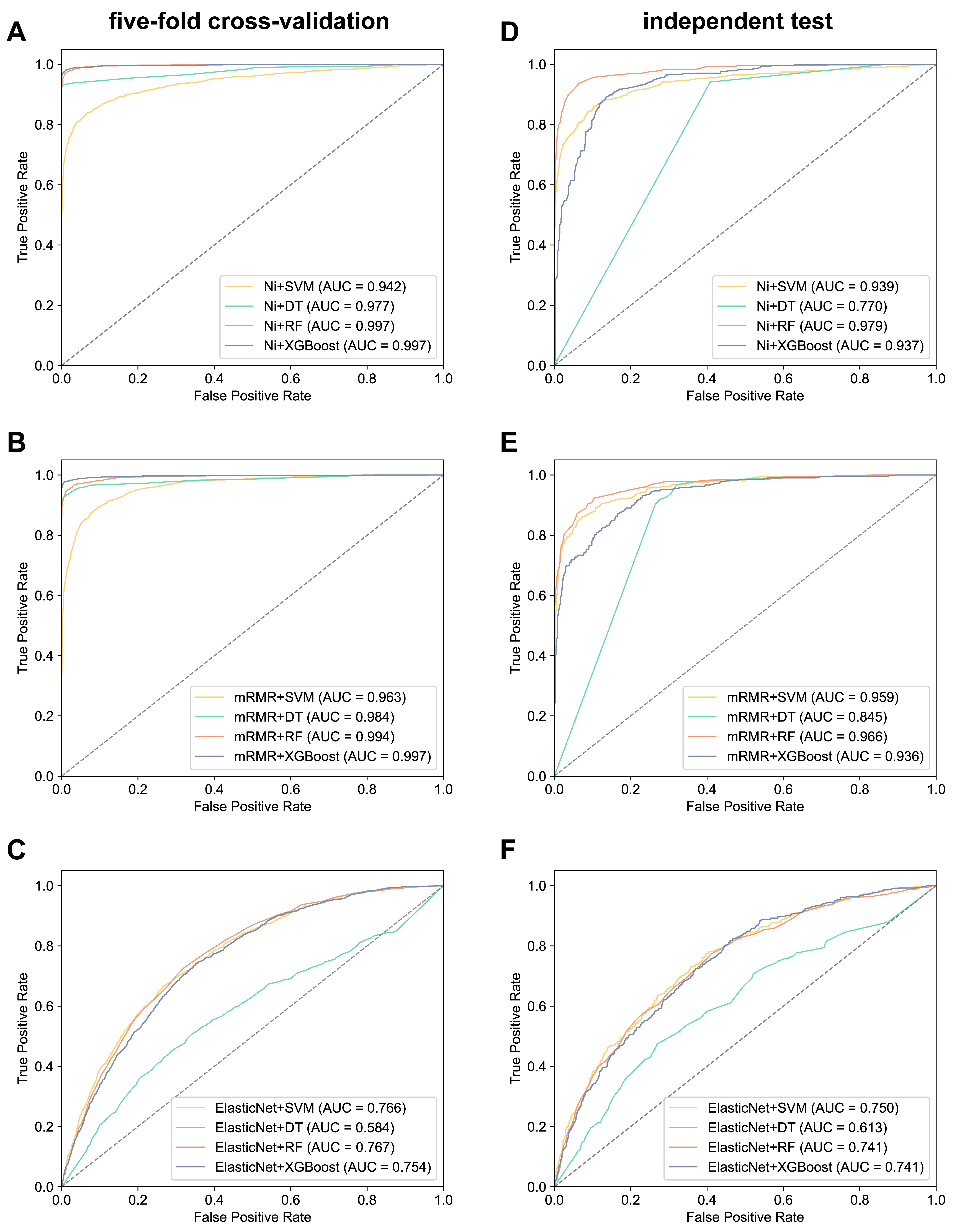 Fig. 3.
ROC curves of different feature selection methods and classifiers for A. thaliana. (A–C) Five-fold cross-validation. (D–F) independent test. ‘Ni’ in (A) and (D) is an abbreviation for Null importances. ROC, Receiver Operating Characteristic.
The datasets for A. thaliana and H. sapiens are unbalanced,
with A. thaliana in particular having a 1:3 ratio of positive to
negative samples. Directly training the model could compromise its
generalizability and robustness. We therefore employed the Null importances+RF
method in A. thaliana to compare model performance with and without
SMOTE. Fig. 4 shows a comparison of the evaluation metrics between the original
dataset and the SMOTE-enhanced model. The MCC for training set cross-validation
with SMOTE (0.962) was not significantly different to the MCC without SMOTE
(0.980) (paired T-test on five metrics, p-value = 0.0506
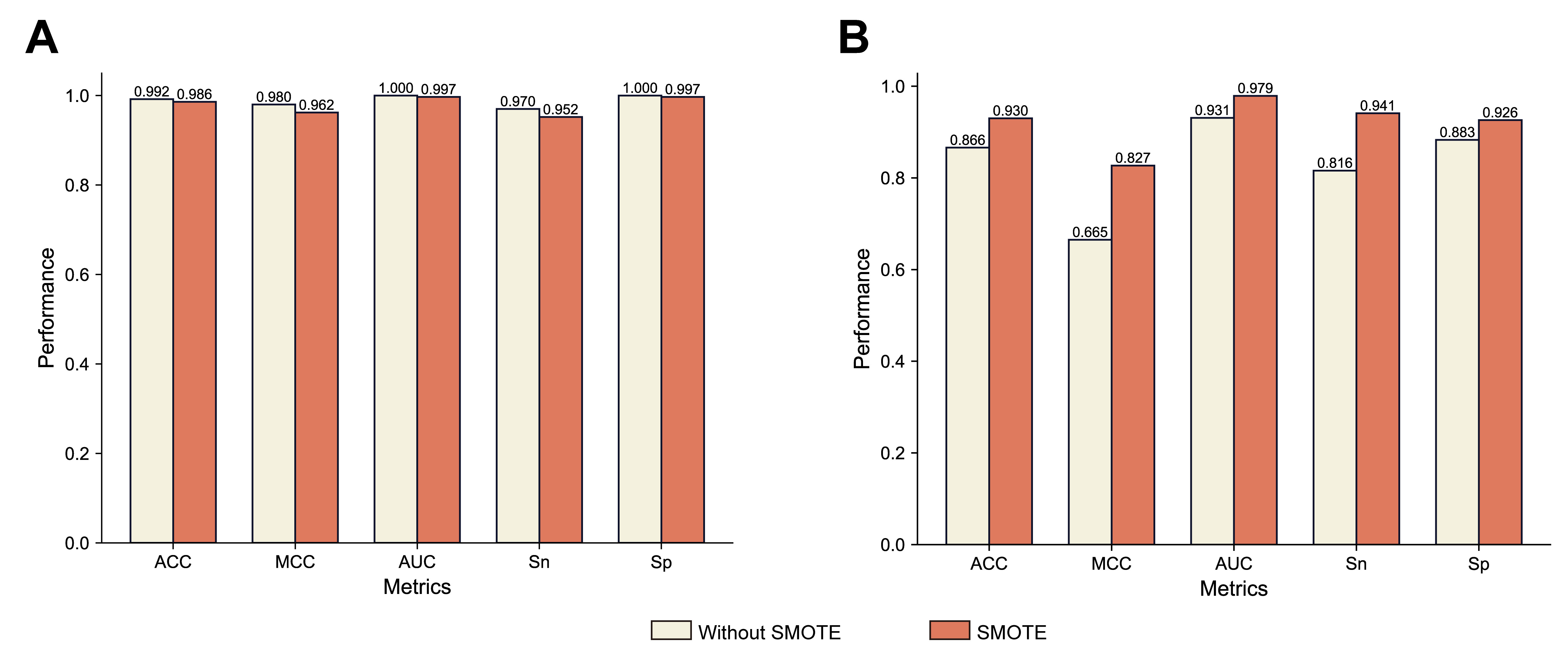 Fig. 4.
Performance comparison between using SMOTE and stratified sampling, and not using SMOTE and stratified sampling in the A. thaliana dataset. (A) Five-fold cross validation. (B) Independent test. SMOTE, Synthetic Minority Over-sampling Technique.
Comparative analysis was conducted using independent tests on the A. thaliana dataset to assess the predictive performance of the selected window size (–16~+14) against the window sizes of established models (–10~+10, –13~+13, –20~+20). As shown in Table 3, the proposed model with 31-residue window size (–16~+14) achieved an ACC of 0.930, an MCC of 0.827, and an AUC of 0.979, signifying greater accuracy. These results indicate that an excessively large window could introduce irrelevant information, while an overly short window could lead to insufficient information, thus potentially reducing the prediction accuracy. This outcome confirms the reliability of our selected window size.
| Window size | Feature dimension | ACC | MCC | AUC |
| –10 |
582 | 0.871 | 0.723 | 0.969 |
| –13 |
700 | 0.897 | 0.764 | 0.970 |
| –20 |
895 | 0.918 | 0.798 | 0.971 |
| –16 |
767 | 0.930 | 0.827 | 0.979 |
The preceding analyses showed that utilization of the chi-square test to capture the sequence window, together with integration of the Null importances + SMOTE + RF method, yielded superior performance. Consequently, the prediction models ArUbNiRF and HoUbNiRF were developed for A. thaliana and H. sapiens, respectively, and then benchmarked against established models. For a fair and unbiased comparison, our model was evaluated using identical training and independent test sets as for the other models, with ‘*’ indicating distinct datasets. The performance metrics of established models were compared based on the information provided in the relevant published articles. Due to the absence of cross-validation outcomes in the majority of H. sapiens models, as well as the utilization of different datasets in some models, the present comparison was based solely on independent test results obtained with the H. sapiens dataset. Table 4, Ref. [16, 17, 18, 19], Table 5, Ref. [12, 13, 14, 15, 26] show the results of performance comparisons between our method and previous studies in A. thaliana and H. sapiens datasets.
| Method | ACC | MCC | AUC | Sn | Sp |
| AraUbiSite [17] | 0.818/0.814 | 0.485/0.468 | 0.877/0.868 | 0.533/0.513 | 0.913/0.914 |
| CNN_Binary [18] | 0.854/0.854 | -/- | 0.924/0.921 | 0.881/0.892 | 0.827/0.817 |
| CNN_Property [18] | 0.843/0.855 | -/- | 0.913/0.914 | 0.849/0.887 | 0.836/0.821 |
| SVM_PseAraUbi [16] | 0.908/0.887 | 0.725/0.722 | 0.953/0.942 | 0.927/0.894 | 0.891/0.897 |
| PrUb-EL [19] | 0.910/0.885 | 0.822/0.772 | 0.977/0.960 | 0.916/0.870 | 0.903/0.900 |
| ArUbNiRF | 0.986/0.930 | 0.962/0.827 | 0.997/0.979 | 0.952/0.941 | 0.997/0.926 |
| Method | ACC | MCC | AUC | Sn | Sp |
| UbiProber* [13] | - | 0.673 | 0.782 | - | - |
| hCKSAAP_UbSite [14] | - | - | 0.757 | - | - |
| ESA-UbiSite* [12] | 0.920 | 0.480 | 0.950 | 0.660 | 0.940 |
| HUbipPred [15] | 0.771 | 0.545 | 0.844 | 0.813 | 0.730 |
| Pourmirzaei et al.* [26] | 0.820 | 0.402 | - | - | - |
| HoUbNiRF | 0.891 | 0.781 | 0.956 | 0.893 | 0.888 |
In the five-fold cross-validation of the Arabidopsis training set, all metrics for ArUbNiRF outperformed those of the other five models. The MCC result in particular was excellent, with the score of 0.827 being a 14% improvement over existing methods. Our method also demonstrated clear advantages across various metrics in the independent test. The values for ACC, MCC, AUC, Sn, and Sp were 0.930, 0.827, 0.979, 0.941, and 0.926, respectively, with all metrics outperforming the other five models. Compared to the current best-performing model, PrUb-EL, the ACC, MCC, AUC, Sn, and Sp metrics improved by 4.5%, 5.5%, 1.9%, 7.1%, and 2.6%, respectively. With the H. sapiens dataset, HoUbNiRF was superior to existing methods with regard to MCC, AUC, and Sn. Despite recording the highest values for ACC and Sp, ESA-UbiSite showed an MCC value of only 0.480. It is important to note, however, that different datasets were utilized. For the same dataset, HoUbNiRF was significantly better across all indicators compared to HUbipPred, which is the the current best-performing method. In particular, the MCC of 0.781 with UbNiRF was a remarkable 23.6% improvement. Next, we performed a thorough comparison with established A. thaliana and H. sapiens ubiquitination site prediction models. ArUbNiRF and HoUbNiRF exhibited notable performance advantages, particularly in addressing the challenge of imbalanced positive and negative samples. In addition, we calculated the computational efficiency of the UbNiRF model for reference by researchers who may be interested in practical applications. The program was executed on a Linux system running CentOS 7.2.1511, with a total RAM of 125GB. For the A. thaliana dataset, comprising a training set of 6129 instances and a test set of 2044 instances, the training and test times were 46.4 seconds and 5.4 seconds, respectively. Similarly, for the H. sapiens dataset consisting of a training set of 10267 instances and a test set of 5801 instances, the training and test times were 55.0 seconds and 5.1 seconds, respectively. Further details are provided in Supplementary Table 2.
Cross-species predictive performance was assessed using UbNiRF for each species. As depicted in Table 6, the model showed superior prediction outcomes when trained on species-matched data. However, employing distinct models for predicting ubiquitination sites in different species within the independent test set notably diminished the performance. This highlights the species-specific nature of ArUbNiRF and HoUbNiRF in predicting ubiquitination sites.
| Test | Training model | |
| ArUbNiRF | HoUbNiRF | |
| A.thaliana | 0.827/0.979 | 0.345/0.754 |
| H.sapiens | 0.103/0.564 | 0.781/0.956 |
The results shown in Table 2 indicate that diverse feature selection methods, alongside classifier combinations, markedly influence model performance. Fig. 5 illustrates the proportion of selected versus not selected features across the different feature selection methods in A. thaliana and H. sapiens. Clear distinctions exist among the individual feature selection methods. High-performing models typically select six features, notably favoring the position-specific information feature PWM (excluding position 0), and showing the least preference for the evolution feature PSSM. The Elastic net model performed the worst, selecting only AA531 features. Fig. 6 shows the relative prevalence of individual features within the chosen feature sets of the different feature selection methods. AA531 exhibited the highest prevalence across all methods. However, superior-performing methods typically encompass six distinct features. Hence, to assess the necessity of incorporating six features, we omitted PSSM features and employed the UbNiRF model to predict both A. thaliana and H. sapiens, ensuring uniform feature dimensions (A. thaliana: 767; H. sapiens: 904). Analysis of independent tests (Table 7) revealed a scarcity of features with minimal proportion. In the A. thaliana model, the ACC, MCC, and AUC showed corresponding decreases from 0.930, 0.827, and 0.979 to 0.900, 0.764, and 0.965, respectively. Similarly, for the H. sapiens model, the ACC, MCC, and AUC decreased from 0.891, 0.781, and 0.956 to 0.883, 0.766, and 0.951. Hence, the amalgamation of multiple informative features and subsequent feature selection are imperative.
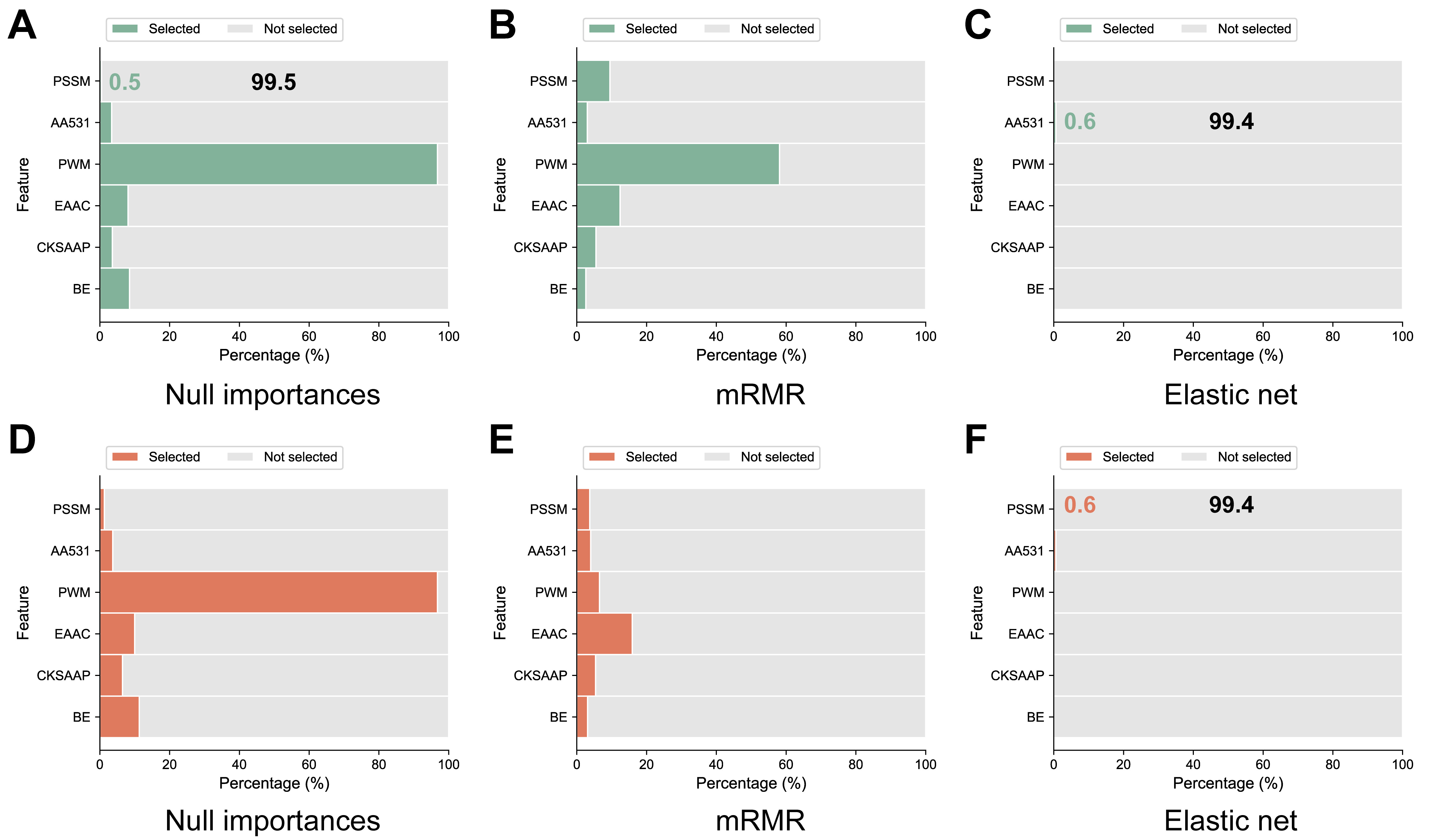 Fig. 5.
Percentage of selected versus unselected features for the three feature selection methods in A. thaliana (A–C), and H. sapiens (D–F).
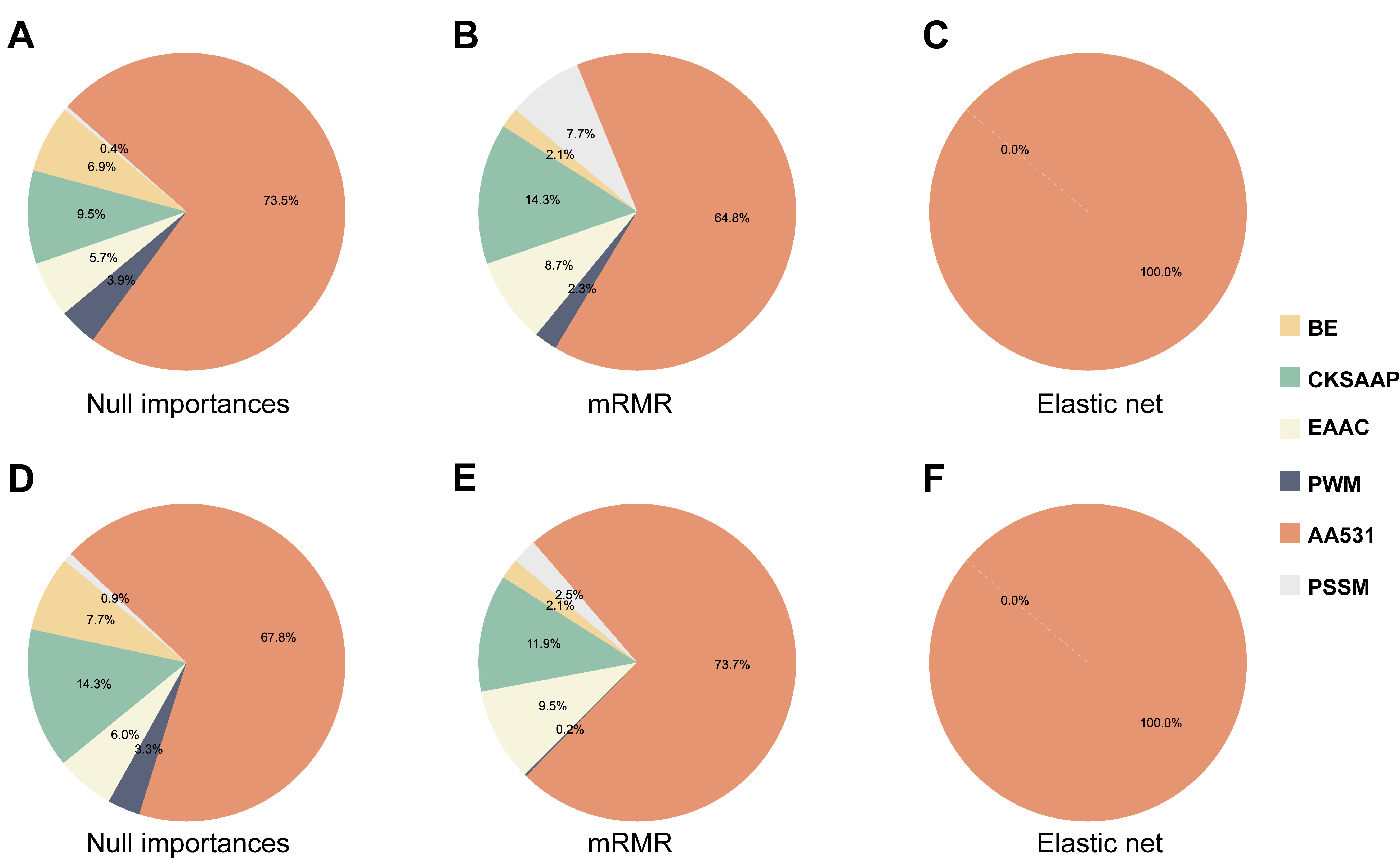 Fig. 6.
Percentage of individual features among selected features based on three feature selection methods in A. thaliana (A–C), and H. sapiens (D–F).
| Number of feature types | ACC | MCC | AUC | Sn | Sp | |
| A. thaliana | 6 (with PSSM) | 0.930 | 0.827 | 0.979 | 0.941 | 0.926 |
| 5 (without PSSM) | 0.900 | 0.764 | 0.965 | 0.930 | 0.890 | |
| H. sapiens | 6 (with PSSM) | 0.891 | 0.781 | 0.956 | 0.893 | 0.888 |
| 5 (without PSSM) | 0.883 | 0.766 | 0.951 | 0.890 | 0.877 |
For each feature, a higher final score indicates a greater contribution to the overall prediction accuracy of the model. Notable differences between A. thaliana and H. sapiens were observed for the contribution of various features to model performance, as illustrated in Fig. 7. In the A. thaliana dataset, the sequence-based EAAC feature showed major importance, possibly due to its direct reflection of amino acid distribution in local protein regions. In particular, the top-ranked feature EAAC_195 (i.e., the frequency of occurrence of arginine ‘R’ at positions –7~–3) is critical for identifying specific Arabidopsis ubiquitination sites. Conversely, in the H. sapiens dataset, the positional feature PWM and the physical and chemical property feature AA531 hold greater importance. The PWM_19 feature (i.e., the frequency of the amino acid at the +2 position) ranked first, indicating a significant contribution to the prediction performance of ubiquitination sites in H. sapiens, as corroborated by Fig. 2B. Although PSSM features in both species constitute a small proportion and are not highly ranked, their contribution to the model was undeniable. As discussed in section 3.6, each type of feature is indispensable.
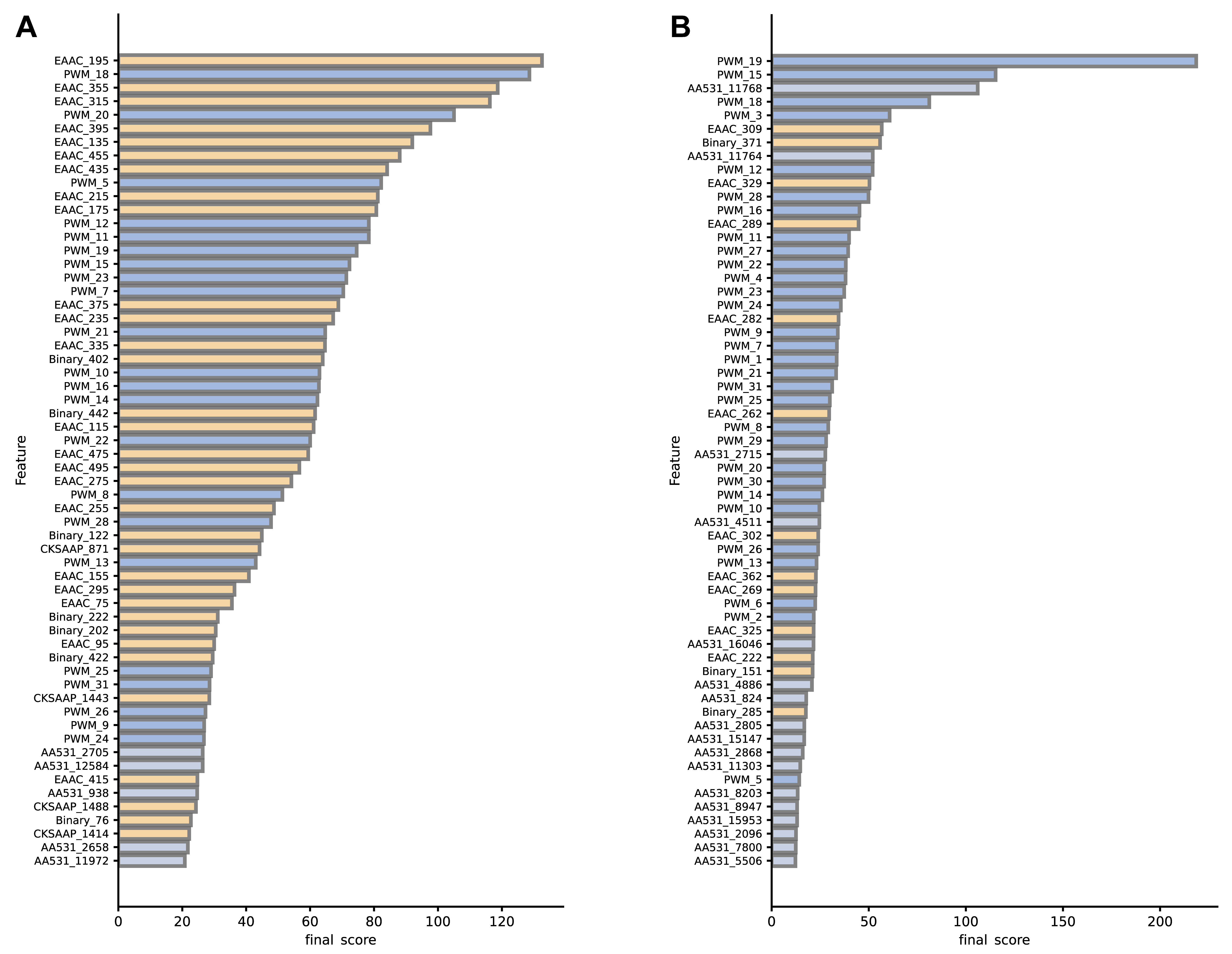 Fig. 7.
Final score for (A) A. thaliana, and (B) H. sapiens training set features (Top 60). Different colors indicate different types of features.
This study presents UbNiRF, a hybrid machine learning framework specifically crafted for predicting ubiquitination sites in both A. thaliana and H. sapiens. Our findings demonstrate the superiority of UbNiRF over current ubiquitination site prediction models across five performance indicators in both A. thaliana and H. sapiens, with particularly good performance for MCC. Furthermore, UbNiRF adeptly captures windows and effectively addresses the imbalance between positive and negative samples. These findings highlight the significance of UbNiRF in reliably predicting ubiquitination sites, which should help to unravel the mechanisms underlying ubiquitination-related biological processes.
Cross-species testing with the ArUbNiRF and HoUbNiRF models validated their species-specificity for the prediction of ubiquitination sites. The use of diverse models for a single species is crucial for accurate prediction of ubiquitination sites. The absence of any of the six features was found to decrease model performance, emphasizing the importance of feature fusion and selection. UbNiRF is therefore a valuable tool for the accurate prediction of ubiquitination sites in both A. thaliana and H. sapiens.
As more and more ubiquitination sites are identified experimentally, some non-ubiquitination sites may in the past have been experimentally identified as ubiquitination sites [48], leading to inaccurate model results. Furthermore, as data continues to accumulate, traditional machine learning may gradually lose its advantages in computational efficiency and predictive capabilities. Therefore, based on large datasets, deep learning algorithms such as the long short-term memory network [49] and convolutional neural network [50] may avoid the effects of empirically extracted features on predictive models. This is expected to further improve the accuracy of the prediction model for ubiquitination sites. The problem of imbalance in the proportion of positive and negative samples in ubiquitination sites is often more serious in practical applications than it was in our dataset. An appropriate data balancing method such as autoencoder [51] or generative adversarial network [52] should be employed in such cases. Further improvements in the prediction of ubiquitination sites are highly significant for gaining a better understanding of important physiological and pathological processes in plants and humans.
AAC, Amino Acid Composition; AAindex, Amino Acid Index; AA531, 531 Properties of Amino Acids; ACC, Accuracy; AUC, Area Under the ROC Curve; A. thaliana, Arabidopsis thaliana; BE, Binary Encoding; BLOSUM62, Blocks Substitution Matrix; ChIP, Chromatin Immunoprecipitation; CKSAAP, Composition of K-Spaced Amino Acid Pair; DT, Decision Tree; EAAC, Enhanced Amino Acid Composition; FPR, False Positive Rate; H. sapiens, Homo sapiens; MCC, Matthews Correlation Coefficient; mRMR, Minimum Redundancy-Maximum Relevance; MS, Mass Spectrometry; PSI-BLAST, Position Specific Iterative-Blast; PSSM, Position-Specific Scoring Matrix; PWM, Position Weight Matrix; RBF, Radial Basis Function; RF, Random Forest; ROC curve: Receiver Operating Characteristic Curve; SMOTE, Synthetic Minority Over-sampling Technique; Sn, Sensitivity; Sp, Specificity; SVM, Support Vector Machine; TPR, True Positive Rate; XGBoost, Extreme Gradient Boosting.
The datasets and source code in this study are available at https://github.com/Hippogriff-ui/UbNiRF.
XL, ZY and YC conceived and designed the experiments. XL performed the experiments. XL, ZY and YC analyzed the data. XL wrote the manuscript. ZY and YC reviewed and edited the manuscript. All authors read and approved the final manuscript. All authors have participated sufficiently in the work and agreed to be accountable for all aspects of the work.
Not applicable.
We appreciate the thorough reading and constructive comments given by the anonymous reviewers that have significantly improved the manuscript.
This research was funded by Special Funds for Construction of Innovative Provinces in Hunan Province, grant number 2021NK1011; Funding for Changsha Science and Technology Plan Project, grant number kh2303010; Medical Scientific Research Foundation of Guangdong Province, grant number A2021284; Guangzhou Basic and Applied Basic Research Foundation, grant number 202201011347.
The authors declare no conflict of interest.
References
Publisher’s Note: IMR Press stays neutral with regard to jurisdictional claims in published maps and institutional affiliations.