


 , Lingyan Du 1,2,*
 , Xi Tan 3, Shirui Song 1,2
1 School of Automation and Information Engineering, Sichuan University of Science and Engineering, 643000 Zigong, Sichuan, China
2 Intelligent Perception and Control Key Laboratory of Sichuan Province, Sichuan University of Science and Engineering, 644000 Yibin, Sichuan, China
3 Zigong Institute of Brain Science, Zigong Mental Health Center, The Zigong Affiliated Hospital of Southwest Medical University, 643020 Zigong, Sichuan, China
Abstract
To examine potential differences in electroencephalogram (EEG) dynamic functional connectivity between patients with major depressive disorder (MDD) and healthy controls (HC), and thereby enhance the effectiveness of depression identification.
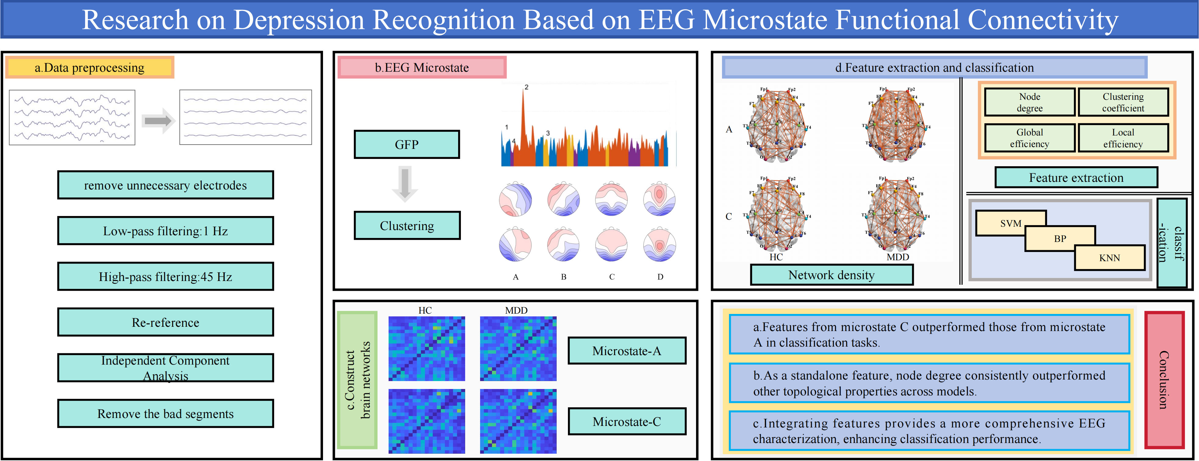
This study presents a novel approach that combines EEG microstate analysis with functional connectivity networks. Resting-state 19-channel EEG data were obtained from 36 participants (17 healthy controls and 19 patients with depression). Through microstate analysis, significant inter-group differences were observed in the average durations of microstates A and C. Subsequently, EEG segments corresponding to microstate classes A and C were extracted. Following the surface Laplacian transformation, the phase locking value (PLV) was applied to construct functional connectivity networks, and their topological characteristics were extracted. Based on the analysis of network indicators (node degree, clustering coefficient, local efficiency, and global efficiency), global and nodal features showing significant group differences were screened and fused with equal weighting. The classification performance of the fused features and individual features was then assessed using three models: Support Vector Machine (SVM), Backpropagation Neural Network (BP), and K-Nearest Neighbors (KNN).
The findings indicate that network features derived from microstate C exhibited higher discriminative ability. Across all classification models, node degree features consistently outperformed other individual topological attributes in recognition accuracy, with the KNN model achieving the highest average accuracy of 96.48%. Furthermore, the fused feature set, incorporating more comprehensive EEG information, showed improved classification performance across all models, exceeding the results obtained using any single feature. The average accuracy reached 97.35% under different model configurations.
Dynamic analysis of brain networks can effectively distinguish patients with depression from healthy controls. This study not only provides a basis for exploring dynamic activities of brain regions associated with depression, but also offers potential objective physiological indicators for disease diagnosis.
Graphical Abstract
Keywords
- depression
- EEG microstates
- brain functional network
- resting state
Depression, as a common mental health disorder, can exert a notable influence on cognitive function [1]. For this reason, it not only affects patients’ quality of life but also places a substantial burden on society [2]. According to the World Health Organization (WHO) Global Burden of Disease report, depression is expected to become the leading cause of global disease burden by 2030 [3]. Despite its high prevalence and serious societal impact, the underlying mechanisms in the brain remain insufficiently understood [4]. Clinically, a depression diagnosis typically relies on a combination of clinical interviews and scale-based assessments [5]. This process is susceptible to subjective influences, such as clinicians’ experience and patients’ self-reporting, and currently lacks objective and quantifiable diagnostic markers. As a result, many researchers have focused on brain imaging technologies, aiming to provide more objective and quantitative physiological indicators for conventional diagnosis. Electroencephalogram (EEG), an important technique for investigating brain functional activity, offers advantages such as cost-effectiveness, portability, non-invasiveness, and ease of operation [6, 7]. By recording electrical potentials generated by neural activity via scalp electrodes, EEG achieves an extremely high temporal resolution [8]. These features make it widely applicable for studying the spatiotemporal properties of neural electrical activity. At present, EEG technology is actively used to explore the pathogenesis of psychiatric disorders and to identify biomarkers, thereby providing valuable insights for diagnostic and therapeutic strategies for related conditions [9].
Research suggests that the onset of depression is closely associated with abnormal neural activity across multiple brain regions and changes in functional connectivity [10]. Accordingly, analysis of brain functional connectivity helps clarify the mechanisms and patterns underlying psychiatric disorders. For example, EEG studies have shown a significant correlation between depression severity and both global efficiency in the alpha band and network diameter [11]. However, interactions between brain regions are inherently transient and dynamic, and traditional functional connectivity analyses often neglect these time-varying features [12].
To overcome the limitations of static analysis, this study adopts a brain electrical microstate functional connectivity approach. Based on the property of microstates as reliable dynamic representations of the whole-brain network at the millisecond scale, this method can effectively capture transient patterns of brain function, opening a new avenue for extracting dynamic abnormal features in mental disorders such as depression [13]. A previous studies has confirmed the potential of this approach for identifying abnormal brain function. Research has shown that dynamic properties of theta and alpha band brain networks, derived from microstate functional connectivity under psychological load, provide potential biomarkers for cognitive state recognition [14]. Likewise, research on disorders of consciousness have demonstrated that microstate-derived dynamic network features can differentiate between varying levels of impairment, further supporting the general applicability of this method for identifying psychopathological states [15].
Based on this background, this study aims to investigate dynamic abnormal patterns of brain networks in depression using the brain microstate functional connectivity method and to provide biomarkers for accurate identification. Specifically, EEG signals are segmented by fitting microstates, and microstate segments with significant inter-group differences in average duration are identified. Dynamic brain networks are then constructed, and key topological features, including node degree, clustering coefficient, global efficiency, and local efficiency, are extracted. Finally, global features and node features with significant inter-group differences are fused with equal weights. By extracting dynamic functional connectivity features, effective discrimination between patients with depression and healthy controls is achieved, providing objective biomarkers for clinical identification.
To investigate differences in dynamic brain networks between patients with depression and healthy controls, reveal functional relationships between brain regions, and improve the accuracy of depression recognition, the methodological procedure of this study is as follows. First, raw EEG data were preprocessed. Next, microstate analysis was performed on the preprocessed EEG data, and the average duration of microstates in the patient group and control group was compared using the Mann–Whitney U test. EEG segments corresponding to microstates with significant inter-group differences were selected as target data for subsequent analysis. Then, the surface Laplacian transformation was applied to the selected EEG segments, and the phase locking value was used to construct the functional connectivity matrix. The matrix was binarized by applying a threshold. Subsequently, topological features were extracted from the binarized network, including global features (global efficiency) and node features (node degree, local efficiency, and clustering coefficient). Statistical methods were used to screen features showing significant inter-group differences between the patient group and the control group. The selected global and node features were equally weighted and fused to form the final classification feature set. Finally, Support Vector Machine (SVM), Backpropagation Neural Network (BP), and K-Nearest Neighbors (KNN) were used as classification models, and the fused feature set served as input for depression recognition. To assess the generalization ability of the model, 5-fold cross-validation was employed, and average accuracy, average precision, average recall, and average F1 score were calculated and statistically analyzed as performance evaluation indicators of the model, with the flowchart shown in Fig. 1.
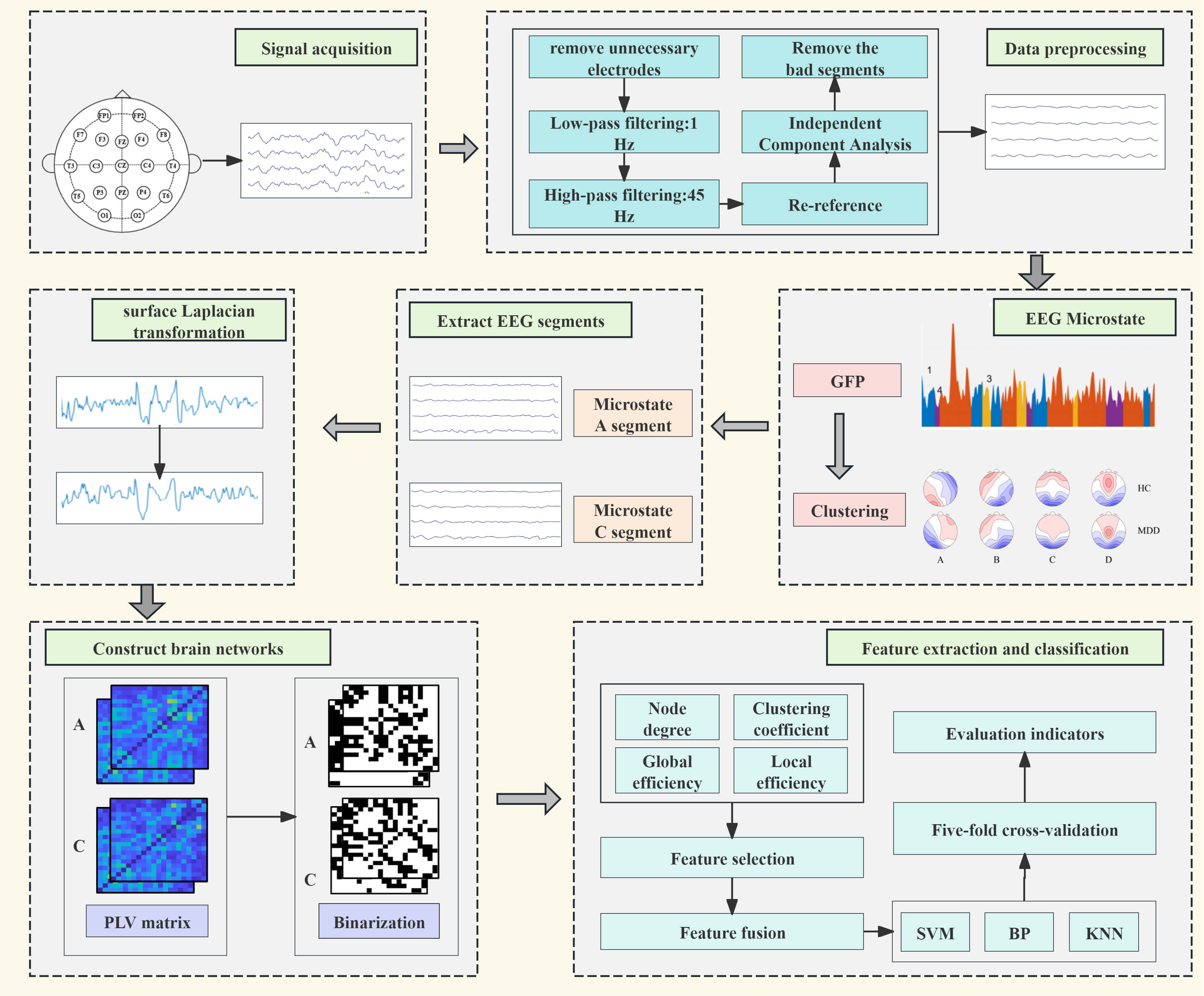 Fig. 1.
Dynamic functional connectivity flowchart. EEG, electroencephalogram; GFP, Global Field Power; PLV, phase locking value; SVM, Support Vector Machine; BP, Backpropagation Neural Network; KNN, K-Nearest Neighbors; FP, frontal pole; F, frontal; FZ, frontal zero; C, central; CZ, central zero; T, temporal; P, parietal; O, occipital; MDD, major depressive disorder; HC, healthy controls.
The resting-state EEG dataset of depression was collected from the Department of Psychiatry of the Fifth People’s Hospital of Zigong City. It included 19 patients with depression (8 males and 11 females) and 17 healthy controls (7 males and 10 females), with ages ranging from 19 to 45 years. All patients were diagnosed by professional doctors according to the depression criteria of the 10th edition of the International Classification of Diseases (ICD-10), and had a clear history of depression. Individuals with severe physical diseases, pregnant or lactating women, and those with other mental disorders were excluded.
The acquisition equipment used was a quantitative digital video EEG system
(SOLAR2848B, Solar Electronic Technologies Co., Ltd., Beijing, China). This
system recorded resting-state scalp potential data from all subjects. It included
24 channels with a sampling frequency of 100 Hz. The impedance of all electrodes
was maintained below 20 k
To obtain relatively clean EEG signals reflecting brain activity, data preprocessing was required. The specific steps included: (1) removing redundant electrodes such as X1 and X2 and retaining signals from the remaining 21 channels, including the bilateral mastoid electrodes A1 and A2; (2) selecting the bilateral mastoids for re-referencing; (3) applying a band-pass filter in the range of 1–45 Hz; (4) using Independent Component Analysis (ICA) to remove artifacts and interference.
EEG microstate analysis was performed using the Microstate 1.0 plugin (version 1.0, EEGLAB toolbox, La Jolla, CA, USA) together with MATLAB-based (R2024b, Mathworks Inc., Natick, MA, USA) custom scripts. Microstate analysis effectively extracts rich spatiotemporal features from EEG signals, characterizing the global functional network dynamics of the brain [16].
The standard analytical procedure included the following steps:
(1) Calculate the Global Field Power (GFP), which measures the instantaneous strength of the brain’s electric field [17]. GFP peaks are often associated with a high signal-to-noise ratio.
(2) Clustering. Based on the calculated GFP data, the K-means algorithm was applied for clustering. Four classical numbers of microstate clusters were selected to obtain EEG microstate topographic maps [18, 19].
(3) Fitting. Using spatial correlation, the clustered template maps were fitted to the original EEG data. Based on the microstates clustered from GFP peak templates, each time point of each subject’s data was assigned to a microstate, and time points were labeled using the best fit.
(4) Analysis of microstate time-domain characteristics. Average duration, time coverage, occurrence frequency, and transition probability were used as features, and EEG segments with statistically significant inter-group differences in average duration were extracted.
Phase locking value (PLV) characterizes undirected functional connectivity by quantifying phase synchrony between neural signals [20, 21]. This metric evaluates the strength of functional connectivity between pairs of electrode signals through phase difference analysis, thereby assessing synchrony in large-scale brain networks [22, 23].
The brain network construction procedure included the following steps:
(1) EEG segment extraction: EEG segments were extracted from microstates showing statistically significant inter-group differences in mean duration.
(2) Spatial enhancement: Surface Laplacian transformation was applied to the extracted EEG data using the Current Source Density (CSD) toolbox (version 1.1, New York State Psychiatric Institute, New York, NY, USA) to improve spatial resolution and reduce volume conduction effects [24].
(3) PLV matrix construction: PLV connectivity matrices were computed for the extracted EEG segments. These matrices were averaged separately for the depression group and the healthy controls group to obtain group-level PLV connectivity matrices.
(4) Threshold binarization: A binarization threshold was selected based on two
criteria: preservation of small-world properties in the resulting network and a
minimum node degree
Brain networks exhibit diverse characteristic parameters. In this study, four features were analyzed: node degree, clustering coefficient, global efficiency, and local efficiency. Node degree, the most basic indicator of network topology, reflects the importance of nodes within a network. The clustering coefficient measures the degree of node aggregation and reflects both local information transfer efficiency and the role of specific nodes in the network [25, 26]. Global efficiency quantifies the speed of information transmission across the entire brain network, representing overall information transfer capacity. Local efficiency assesses information exchange capability and fault tolerance among neighboring nodes, indicating the closeness of connectivity between a node and its adjacent nodes [27].
Classification was performed using SVM, KNN, and BP models. For SVM, a radial basis function kernel was employed with a penalty parameter (C) of 100 and a kernel coefficient (gamma) of 0.1. The BP model used a hidden layer size of 10, a maximum of 500 iterations, and a learning rate of 0.001. For KNN, K was set to 7. Model performance was evaluated using 5-fold cross-validation. Evaluation metrics included average accuracy, precision, recall, and F1 score.
Statistical analysis was conducted using SPSS software (version 27.0, IBM Corp., Chicago, IL, USA). Continuous variables were tested for normality using the Shapiro–Wilk test. The independent-samples t-test was applied to data that followed a normal distribution and showed homogeneity of variance, whereas the Mann–Whitney U test was used for non-normally distributed data. Results for non-normally distributed variables are reported as median (Q1, Q3).
The dataset included 19 patients with major depressive disorder (MDD) and 17 healthy controls (HC). Demographic characteristics are presented in Table 1. Independent sample t-tests indicated that there was no significant difference in age between the two groups (t = 0.079, p = 0.937). Pearson’s chi-square test showed that there was no significant difference in gender distribution between the two groups (t = 0.003, p = 0.955).
| HC (n = 17) | MDD (n = 19) | t/χ2 | p | |
| Age | 29.06 |
29.26 |
0.079 | 0.937 |
| Sex:n (M:F) | 7:10 | 8:11 | 0.003 | 0.955 |
Age was expressed as mean
Based on the Global Explained Variance (GEV) and Cross-Validation (CV) criteria, four classic microstate numbers were selected. This number is also consistent with the classic microstate numbers adopted in most of the literature in this research field, which is conducive to the comparison and verification of the results, and their fitting results are illustrated in Fig. 2.
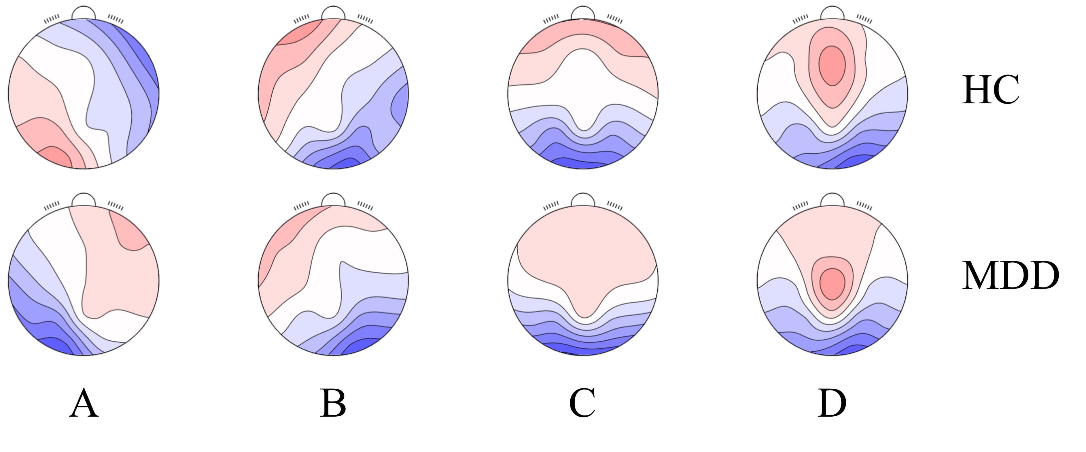 Fig. 2.
Microstate fitting results. (A) represents microstate A; (B) represents microstate B; (C) represents microstate C; (D) represents microstate D.
Statistical analysis was conducted on the average duration, time coverage, and
occurrence frequency. The depression group and the healthy controls did not
conform to the normal distribution, so the Mann-Whitney U test was used, where U
is the statistic of this test and Z is the standardization of U, used to
calculate the two-tailed p value. When p
| Category | Z | p | ||
| HC (n = 17) | MDD (n = 19) | |||
| A_Duration | 121.33 (107.92, 132.83) | 83.37 (76.84, 86.29) | 4.959 | |
| B_Duration | 77.86 (74.91, 97.73) | 83.40 (78.14, 95.15) | 0.491 | 0.623 |
| C_Duration | 81.93 (75.41, 85.74) | 101.43 (92.65, 108.75) | 3.470 | |
| D_Duration | 71.84 (69.22, 85.18) | 71.75 (64.99, 114.32) | 0.143 | 0.887 |
All duration values are presented as median (interquartile range, IQR).
The nomenclature of the electrode sites is as follows: FP (frontal pole), F (frontal), FZ (frontal zero), C (central), CZ (central zero), T (temporal), P (parietal), and O (occipital). The data from 19 channels were divided into different brain regions. The prefrontal area includes: FP1, FP2; the frontal area includes: F3, F7, FZ, F4, F8; the central area includes: C3, CZ, C4; the temporal area includes: T3, T4; the parietal area includes: T5, T6, P3, P4, PZ; the occipital area includes: O1, O2. The schematic diagram of brain regions is shown in Fig. 3.
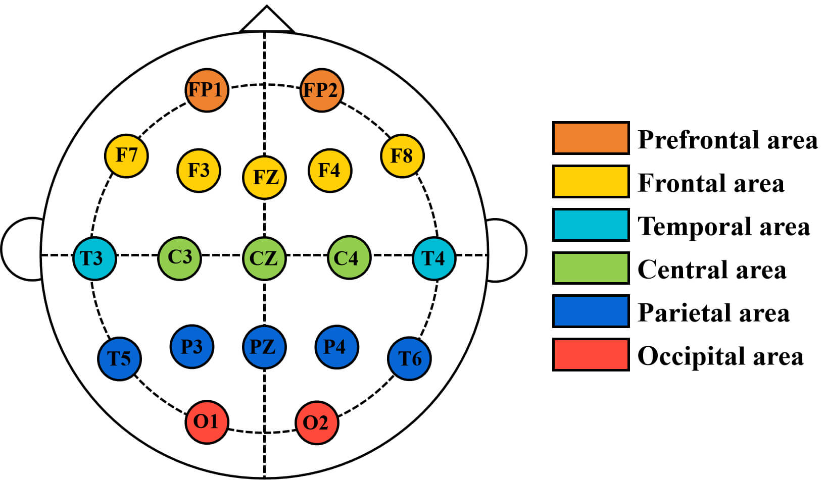 Fig. 3.
Schematic diagram of brain regions.
Whole-scalp EEG data underwent surface Laplacian transformation to compute the radial CSD at each electrode. This spatial filtering approach attenuated volume conduction effects, significantly reducing functional connectivity values measured by PLV and partially eliminating shared components across electrodes. To balance sample distribution and ensure adequate data volume for subsequent classification tasks, the first 2 minutes of resting-state EEG per subject were segmented into non-overlapping 30-second epochs. For microstate class A, this yielded 66 segments from the healthy controls HC group and 66 from the MDD group (n = 132). For microstate class C, 49 segments came from HC and 64 from MDD (n = 113). For each microstate class, PLV-based functional connectivity matrices were constructed from all channel data within each epoch. Group-averaged PLV matrices were then derived for HC and MDD cohorts, as illustrated in Fig. 4.
 Fig. 4.
Average PLV matrix. Each row and column of the matrix represents 19 channels. (A,B) Show the microstate A segments extracted from the EEG, while (C,D) represent the microstate C segments extracted from the EEG. (A) Microstate A - healthy controls. (B) Microstate A - depression group. (C) Microstate C - healthy controls. (D) Microstate C - depression group. Chan, channels.
The functional connectivity matrices were binarized based on a threshold selection principle, and we adopted a relatively small uniform threshold. This choice was based on the following: the CSD transformation has significantly reduced the false high connections caused by volume conduction. A lower threshold can more conservatively and effectively exclude noise-driven weak connections, thereby ensuring that the observed inter-group network differences are more likely to result from genuine neurophysiological distinctions. The specific thresholds for each microstate are defined as follows: For microstate A, the maximum connectivity value was 0.26 in the depression group and 0.29 in healthy controls; thus, a threshold of 0.26 was applied. For microstate C, the maximum connectivity value was 0.29 in the depression group and 0.26 in controls; consequently, the threshold was set to 0.26. Fig. 5 demonstrates that after binarization, both microstate A and C exhibited greater connection density in the depression group compared to healthy controls.
 Fig. 5.
Binary matrix. Each row and column of the matrix represents 19 channels. (A,B) Show the microstate A segments extracted from the EEG, while (C,D) represent the microstate C segments extracted from the EEG. (A) Microstate A - healthy controls. (B) Microstate A - depression group. (C) Microstate C - healthy controls. (D) Microstate C - depression group.
To investigate interregional connection density differences, functional connectivity patterns were visualized using the BrainNet Viewer toolbox (1.6, Beijing Normal University, Beijing, China) [29]. The topographical distribution of these connections is presented in Fig. 6. Results demonstrate that the depression group exhibited significantly higher global connection density compared to healthy controls. Specifically, in microstate A, density differences localized primarily to frontal, central, and parietal regions. In microstate C, increased density in the depression group concentrated in the central region, whereas no significant intergroup differences emerged in other regions.
 Fig. 6.
Brain network connectivity diagram. Figures (A) and (B) show the microstate A segments extracted from the EEG, while (C) and (D) represent the microstate C segments extracted from the EEG. (A) Microstate A - healthy controls. (B) Microstate A - depression group. (C) Microstate C - healthy controls. (D) Microstate C - depression group.
(1) Node degree
The Shapiro-Wilk test indicated that the node degree feature was not normally
distributed; therefore, the Mann-Whitney U test was used. Although the depression
group exhibited a higher average node degree than the healthy controls in both
microstates A and C, the difference reached statistical significance only in
microstate C (p
Analysis of channels across different brain regions (Fig. 7) further detailed
differences between the depression group and healthy controls. In microstate A,
the depression group showed significantly increased activity at frontal channel
F7 (p = 0.026), central channels C3 (p
 Fig. 7.
Node degree. (A) Microstate A. (B) Microstate C. * indicates
p
(2) Clustering coefficient
The Shapiro-Wilk test indicated that the clustering coefficient features were
not normally distributed; therefore, the Mann-Whitney U test was employed. For
microstate A, the healthy controls exhibited a higher overall clustering
coefficient than the depression group, though this difference did not reach
statistical significance. Conversely, for microstate C, the depression group
demonstrated a significantly higher overall clustering coefficient than the
healthy controls (p
Channel analysis across brain regions (Fig. 8) revealed distinct differences
between the depression group and healthy controls during microstate classes. In
microstate A, the depression group exhibited significantly increased activity at
the parietal PZ channel (p
 Fig. 8.
Clustering coefficient. (A) Microstate A. (B) Microstate C. *
indicates p
(3) Global efficiency
The Shapiro-Wilk test indicated that global efficiency was not normally
distributed, so the Mann-Whitney U test was employed. As shown in Fig. 9,
depression patients exhibited higher global efficiency than healthy controls
during microstates A and C, with statistically significant inter-group
differences in microstate C (p
 Fig. 9.
Global efficiency. *** indicates p
(4) Local efficiency
Shapiro-Wilk tests indicated that local efficiency measures in both the
depression and healthy controls violated the normality assumption; a Mann-Whitney
U test was employed. During microstates A and C, the depression group exhibited
significantly higher global local efficiency than healthy controls. Notably, in
microstate C, this intergroup difference reached statistical significance
(p
Analysis of EEG channels across brain regions (Fig. 10) revealed distinct
patterns in depression patients compared to healthy controls during microstate
classes. In microstate A, the depression group exhibited significantly increased
activity at the parietal T5 channel (p = 0.008), while showing
significantly decreased activity at the temporal T4 (p
 Fig. 10.
Local efficiency. (A) Microstate A. (B) Microstate C. *
indicates p
Dynamic functional connectivity provides a more effective approach for capturing
time-varying neural interactions. We extracted four graph-theoretical features:
node degree, clustering coefficient, global efficiency, and local efficiency.
Significantly different global and nodal features were selected and equally
weighted for fusion. The fused features were then classified using SVM, BP and
KNN models. In microstate A, node degree, clustering coefficient, and local
efficiency each exhibited dimensions of 19 channels
| Classifier | Feature | Average accuracy rate (%) | Average precision (%) | Average recall rate (%) | Average F1 score (%) |
| SVM | node degree | 87.86 | 87.99 | 87.62 | 87.70 |
| clustering coefficient | 72.05 | 72.61 | 71.66 | 71.60 | |
| global efficiency | 48.38 | 52.87 | 49.51 | 43.26 | |
| local efficiency | 74.33 | 74.29 | 73.67 | 73.61 | |
| Integrated Features | 88.63 | 88.55 | 88.50 | 88.50 | |
| BP | node degree | 85.67 | 85.76 | 85.35 | 85.33 |
| clustering coefficient | 71.28 | 71.43 | 70.91 | 70.81 | |
| global efficiency | 55.41 | 54.00 | 54.39 | 53.06 | |
| local efficiency | 75.75 | 76.26 | 75.34 | 75.22 | |
| Integrated Features | 90.85 | 90.94 | 90.62 | 90.73 | |
| KNN | node degree | 85.58 | 85.89 | 85.65 | 85.48 |
| clustering coefficient | 80.31 | 80.64 | 79.89 | 79.89 | |
| global efficiency | 50.77 | 50.42 | 50.68 | 48.17 | |
| local efficiency | 74.25 | 74.46 | 73.61 | 73.55 | |
| Integrated Features | 88.63 | 88.95 | 88.33 | 88.40 |
| Classifier | Feature | Average accuracy rate (%) | Average precision (%) | Average recall rate (%) | Average F1 score (%) |
| SVM | node degree | 95.57 | 95.09 | 95.65 | 95.26 |
| clustering coefficient | 86.72 | 86.77 | 85.17 | 85.77 | |
| global efficiency | 69.88 | 71.85 | 68.20 | 66.85 | |
| local efficiency | 88.42 | 87.85 | 87.67 | 87.65 | |
| Integrated Features | 97.35 | 97.66 | 96.86 | 97.11 | |
| BP | node degree | 96.44 | 96.00 | 96.42 | 96.13 |
| clustering coefficient | 84.98 | 83.85 | 82.82 | 83.14 | |
| global efficiency | 67.15 | 68.13 | 68.07 | 66.25 | |
| local efficiency | 88.50 | 88.76 | 87.00 | 87.59 | |
| Integrated Features | 97.35 | 97.37 | 97.22 | 97.16 | |
| KNN | node degree | 96.48 | 96.17 | 96.40 | 96.19 |
| clustering coefficient | 88.46 | 90.52 | 86.87 | 87.58 | |
| global efficiency | 69.88 | 70.97 | 68.25 | 67.37 | |
| local efficiency | 87.51 | 87.10 | 87.23 | 86.82 | |
| Integrated Features | 97.35 | 97.99 | 96.46 | 97.08 |
This study has certain limitations. First, the EEG sample size is relatively small, while the classification model involves high-dimensional features. This combination introduces a potential risk of overfitting, meaning that the high classification accuracy observed may not generalize beyond the current dataset. Although cross-validation was used to reduce this risk, model performance was not tested on an independent external dataset. Second, EEG results may be affected by factors such as data preprocessing strategies and control of confounding variables. Finally, the current research aims to use the preliminary Mann-Whitney U test to screen out valuable candidate indicators from the relevant features, reduce the dimension of the fused features, and provide input for machine learning. Essentially, it is exploratory in nature. Therefore, future studies should focus on validating the present findings using larger datasets to improve reliability and generalizability and reduce overfitting risk, while also optimizing experimental design and standardizing preprocessing procedures to enhance comparability across studies.
This study used a combined microstate and functional connectivity approach to investigate dynamic inter-regional brain connectivity. Microstate analysis revealed significant group differences in the average duration, temporal coverage, and occurrence frequency for microstates A and C. In line with established neurophysiological models, microstate A is related to the auditory network, microstate B to the visual network, microstate C to the salience network, and microstate D to the attention network [30, 31, 32]. This suggests the presence of abnormalities in the auditory network and internal perceptual processing in depression. In addition, previous studies have shown that EEG microstates can serve as biomarkers for the auxiliary diagnosis of depression or for assessing treatment efficacy. For example, Peng et al. [33] reported that EEG microstates, especially C and D, may function as biomarkers for depression. Che et al. [34] further found that microstate C is associated with anhedonia and may represent a reliable biomarker for transcranial magnetic stimulation (TMS) treatment in depression.
Brain networks were constructed using segments from microstates A and C, which showed significant differences in average duration. Analysis of connection density indicated that patients with depression exhibited higher connectivity than healthy controls, particularly in central regions, where connections were notably denser. This finding is consistent with the overall trend reported by Hasanzadeh et al. [35], showing that patients with depression have higher brain network density than healthy controls across multiple frequency bands.
Analysis of brain network parameters showed the following: (1) Nodal connectivity was higher in patients with depression than in healthy controls, with statistically significant group differences observed only in microstate C, suggesting hyperactive neural engagement during salience-network-related states. For microstate A, significant between-group differences in node degree were found in the frontal region (F7, F8), central region (C3, CZ), temporal region (T3, T4), and parietal region (P3, T6, PZ). For microstate C, significant differences were observed in the frontal region (F3, FZ), central region (C3, CZ), temporal region (T3, T4), and parietal region (P3, T5, T6, PZ). (2) In microstate A, the clustering coefficient was higher in healthy controls than in the depression group, whereas in microstate C, the clustering coefficient was significantly higher in the depression group. This pattern suggests that healthy controls may show stronger information transmission and processing during microstate A, while patients with depression exhibit stronger capabilities during microstate C. For microstate A, significant differences in clustering coefficient were observed at electrodes in the prefrontal area (FP2), frontal area (F8), temporal area (T4), and parietal area (T6, P3, P4, PZ). For microstate C, significant differences were detected in the frontal area (FZ), central area (C4, CZ), temporal area (T3, T4), parietal area (T6, PZ), and occipital area (O1). (3) Global efficiency was higher in the depression group than in healthy controls for both microstates A and C, but this difference reached statistical significance only in microstate C. This indicates faster whole-brain information transmission in patients with depression during these microstates. (4) Local efficiency was also higher in the depression group for both microstates A and C, with statistically significant differences again limited to microstate C. This suggests enhanced local information transfer within brain regions in patients with depression. For microstate A, significant differences in local efficiency were found in the temporal region (T4) and parietal region (T5, T6, P3, P4, PZ). For microstate C, significant differences were observed in the frontal region (FZ), central region (C4, CZ), temporal region (T3, T4), parietal region (T5, PZ), and occipital region (O1).
The classification results show that brain network features derived from microstate C have stronger discriminative ability. Among individual topological features, node degree consistently performed better than other features across all classification models, with the KNN classifier achieving an average accuracy of 96.48%. Feature fusion captured EEG information in a more comprehensive manner and further improved classification performance, reaching an average accuracy of 97.35%, which exceeded that of any single-feature approach.
In summary, functional connectivity measures derived from EEG microstates demonstrate strong discriminative power between patients with depression and healthy controls. These measures provide objective and quantifiable indicators for clinical diagnosis and treatment monitoring and may serve as a useful reference for depression management.
From the perspective of dynamic functional connectivity between brain regions, this study divided the original EEG signals into four stages based on microstates and extracted EEG segments showing inter-group differences in average duration to construct brain networks. The results indicated significant inter-group differences in the average duration of microstates A and C in depression. For brain network feature extraction, node degree, clustering coefficient, global efficiency, and local efficiency were selected, and global and nodal features with significant inter-group differences were screened and fused with equal weights. Classification results showed that networks constructed from microstate C achieved higher average accuracy and recognition performance than those from microstate A. Among individual features, node degree demonstrated better discriminative ability, while fused features further enhanced classification performance. These findings indicate that dynamic brain network analysis can effectively distinguish patients with depression from healthy controls. This study not only provides a basis for exploring dynamic brain activity related to depression but also offers potential objective physiological indicators for disease diagnosis.
The dataset we possess contains sensitive information, such as the fundamental demographic details of patients diagnosed with depression. In accordance with the ethical agreement established with the hospital, please contact the corresponding author to request access to the dataset.
ZT and LD designed the research study. ZT, LD and SS performed the research. ZT, SS, XT analyzed the data. ZT, XT and LD wrote the manuscript. All authors contributed to editorial changes in the manuscript. All authors read and approved the final manuscript. All authors have participated sufficiently in the work and agreed to be accountable for all aspects of the work.
The study was conducted in accordance with the Declaration of Helsinki. The research protocol was approved by the Ethics Committee of Zigong Mental Health Center (Ethic Approval Number: 202400717), and all of the participants provided signed informed consent.
Not applicable.
This research was funded by the National Natural Science Youth Foundation of China (Grant No. 12304469) and the Science and Technology Bureau of Zigong City (Grant No. 2024-NKY-03-04).
The authors declare no conflict of interest.
References
Publisher’s Note: IMR Press stays neutral with regard to jurisdictional claims in published maps and institutional affiliations.