
- Academic Editors
Background: Autism Spectrum Disorder (ASD) is a complex
neurodevelopment disease characterized by impaired social and cognitive
abilities. Despite its prevalence, reliable biomarkers for identifying
individuals with ASD are lacking. Recent studies have suggested that alterations
in the functional connectivity of the brain in ASD patients could serve as
potential indicators. However, previous research focused on static
functional-connectivity analysis, neglecting temporal dynamics and spatial
interactions. To address this gap, our study integrated dynamic functional
connectivity, local graph-theory indicators, and a feature-selection and ranking
approach to identify biomarkers for ASD diagnosis. Methods: The
demographic information, as well as resting and sleeping electroencephalography
(EEG) data, were collected from 20 ASD patients and 25 controls. EEG data were
pre-processed and segmented into five sub-bands (Delta, Theta, Alpha-1, Alpha-2,
and Beta). Functional-connection matrices were created by calculating coherence,
and static-node-strength indicators were determined for each channel. A
sliding-window approach, with varying widths and moving steps, was used to scan
the EEG series; dynamic local graph-theory indicators were computed, including
mean, standard deviation, median, inter-quartile range, kurtosis, and skewness of
the node strength. This resulted in 95 features (5 sub-bands
The complex neurological condition known as Autism Spectrum Disorder (ASD) can lead patients to exhibit repetitive and limited activities that impede their day-to-day functioning [1]. When Kanner [2] initially described ASD in 1943, he identified two key characteristics: abnormal and repetitive sensory-motor activities; and social communication impairments. Early detection and treatment could significantly mitigate the impact of later symptoms [3]. However, traditional diagnosis heavily relies on clinical-symptom questionnaires, increasing the risk of widespread misdiagnosis [4, 5]. The overlapping and unclear symptoms of ASD make traditional identification challenging. Thus, it is crucial to identify biomarkers related to symptoms in order to assist in clinical diagnosis and to provide insight into the mechanisms underlying ASD [6].
Previous studies have focused on searches for fundamental biomarkers of brain functional connectivity. Because of its great temporal resolution and ease of use, electroencephalography (EEG) is typically used in these types of studies. An essential characteristic of ASD, according to electronic physiology studies, is abnormal functional neural circuits [7, 8]. ASD individuals retain an excessive number of synaptic connections because they do not experience the regular pruning of synapses during childhood [9]. It has been argued that an excess of neurons creates local functional over-connectivity. The statistical dependence of signals, such as the coherence at a certain frequency, between two brain regions, over time, is referred to as functional connectivity. EEG and magnetoencephalography (MEG) can be used to determine functional connectivity. By using millisecond temporal resolution, EEG signals reflect an approximate measure of postsynaptic pyramidal cell activity [10]. Although some studies produced inconsistent or even contradictory results [10, 11, 12, 13], the most widely accepted finding, currently, is that patients with ASD have lower level of long-range functional connectivity (e.g., between frontal and parietal regions) and a higher level of short-range connectivity (e.g., within frontal regions) [14]. Previous studies have mostly focused on the functional connectivity of a particular pair of regions; however, two-region connectivity is considered a low-order signal because it is considered to contain relatively little information, and cannot account for interactions from other regions [15]. In order to overcome this limitation, the topological characteristics of the entire brain functional-connection network were proposed to be described by complex network analysis, also known as graph-theory analysis [16, 17].
The entire brain functional-connection network can be viewed as a graph in the graph-theory approach, with the EEG channels acting as the nodes, and the connectivity strength between channel pairs acting as the edges. An array of graph-theory indicators, which may be further classified into global and local indicators, could characterize the topological characteristics of the entire brain network. The global indicators include small-world, global efficiency, global degree, and so on, which describe the topological traits of the whole network; local indicators, such as node degree (or node strength), and node efficiency, describe the function of a specific node (or a brain region in the context of brain network) in a network [18]. Because ASD is sometimes regarded as a “disconnection syndrome”, graph-theory research of brain networks is especially suitable for studying ASD [19]. Preschool-aged ASD patients showed higher node efficiency of the right lingual gyrus and a higher node degree of the right medial frontal gyrus, than did normal controls [20]. This suggests that graph-theory indicators could be useful biomarkers for the early diagnosis of ASD patients. Certain global measures, such as average node degree, are the average of their corresponding local indicators; however, the averaging process may obliterate important information necessary for diagnosis. Results suggested that there was only a significant difference in local graph-theory indicators between ASD patients and controls, not in global ones [20], which meant that some local-network topological qualities experienced modifications, and that those changes might not be discovered by global graph-theory indicators. However, it is possible to determine which features are most relevant for the disease diagnosis in a data-driven manner by fusing local graph theory with feature selection and ranking approaches [21].
Previous research tended to treat the EEG data as static. It was noted that the reason for the paradoxical results from static functional-connectivity analysis might be from not measuring instantaneous dynamic changes in EEG connectivity [22], since EEG signals are characteristically unstable. Results from a micro-state analysis showed that EEG shifts its states in 100 ms [23]. In order to capture the dynamic characteristics of the EEG signal, a dynamic Functional-Connectivity Analysis (dFCA) was proposed. In dFCA, the EEG signal is separated into numerous epochs by a sliding window, and the variability among these epochs can be computed [24]. Functional magnetic resonance imaging (fMRI) was employed in a study of 102 normally developing control children and 105 children with ASD [25]. According to the findings, the children with ASD showed less variability in the fusiform gyrus-inferior temporal gyrus connectivity, and more variability in the anterior cingulate cortex-medial prefrontal cortex connectivity, than did the controls. Dynamic functional connectivity is useful in the identification of several illnesses, including ASD [26]. It may also reflect the dynamic reconfiguration of various regions over time, which may further reflect the brain’s flexibility and adaptability. One study [23] employed the sliding-window method to divide the EEG signal of ASD patients and controls into several epochs. Then, the researchers used k-mean clustering to divide these epochs into four states. The results showed that, although static functional connectivity did not reveal the difference, the pattern of the two states was significantly different in ASD patients and controls, suggesting that useful information may be present in the process of state shift in ASD. Features from dynamic functional connectivity were found to achieve a higher classification accuracy for diagnosing ASD children, validating the special benefit of dynamic functional connectivity in diagnosing ASD patients [27]. The researchers did this by combining the dynamic functional-connectivity calculation with a multiple-kernel support vector machine model.
In the present study, we attempted to combine the benefits of dynamic functional connectivity and local graph-theory indicators. Using a data-driven method, we sought to identify the most discriminative features for ASD diagnosis by utilizing feature selection and ranking techniques. Furthermore, we attempted to assess the effectiveness of different window widths in dynamic functional-connectivity analysis to provide empirical information for the best window-width selection for subsequent studies. The workflow is depicted in Fig. 1.
 Fig. 1.
The work flow of the research project. EEG, electroencephalography; SVM, support vector machine; RFE, recursive feature elimination. The * means the process of multipling. In other words, each channal could provide 5 features, and finally obtain total 95 features (19 multipling 5 equal to 95).
The EEG data and diagnosis details were obtained from Zhongshan Bo’ai Hospital’s internal medical record system, located in Zhongshan City, China. The inclusion criteria for the ASD patient group were: (1) diagnosed as ASD according to Diagnostic and Statistical Manual of Mental Disorders-V (DSM-V) criteria; and (2) aged 1–6 years. Exclusion criteria for the ASD patients were: (1) a history of epilepsy seizures; and (2) patients who had suffered from other neurological, developmental diseases, or extra-cranial injury. Controls were selected from children who were hospitalized for non-neurological disease, e.g., diarrhea, in the same age range. Altogether, 20 ASD patients and 25 health controls were recruited. Informed consent was obtained from the parents of all subjects involved in the study.
Nicolet EEG machines (Host: PN100973M ; Amplifier: V32-09472364, Natus Medical Incorporated, Pleasanton, CA, USA) with a 125-Hz sample rate were used to record the resting EEG signals of the subjects when they were sleeping. According to the international 10–20 montage system [28], a total of 19 channels (Fp1, Fp2, F7, F3, Fz, F4, F8, T3, C3, Cz, C4, T4, T5, P3, Pz, P4, T6, O1, and O2) were fastened onto the patient’s scalp [29]. The following were the EEG pre-processing steps: (1) the average re-reference and band-pass filtering between 0.1 Hz and 45 Hz were carried out for EEG signals, using the “pop_eegfiltnew” function in EEGLab toolbox v.14.1.2.0 (https://sccn.ucsd.edu/eeglab/index.php) [30] to remove artifacts; (2) independent component analysis (ICA) was carried out to remove artifacts originating from eye and muscle movement. The IClabel plug-in unit (https://labeling.ucsd.edu/auth/login) [31] carried out the identification of these components; (3) Manual elimination of the problematic segments from the eye, muscle, or body’s gross movement, that ICA was unable to identify; (4) recheck, by two experts, of the pre-processed EEG data, and extraction of the 100-s signal from the beginning of the pre-processed EEG signal; and (5) EEGs were further filtered into 5 frequency sub-bands, Delta (0.5–4 Hz), Theta (4–8 Hz), Alpha-1 (8–10 Hz), Alpha-2 (10–12 Hz), Beta (12–30 Hz) by the “pop_eegfiltnew” function in EEGLab. The pre-processing described above was carried out in Matlab v. 2019a using the EEGLab toolbox v.14.1.2.0 (https://sccn.ucsd.edu/eeglab/index.php).
In order to investigate the linear relationship between two signals in the fixed frequency, we computed magnitude-squared coherence, or coherence. By assuming that Y (t) and X (t) represent EEG signals in two brain regions or regions of interest (ROIs), first Y (t) and X (t) were converted from the time domain to the frequency domain using a fast Fourier transform:
Then, for each frequency point f, power spectral densities
S
A connection matrix could be formed once all of the functional connectivity had been computed for each pair of ROIs. It is important to apply a threshold, in order to eliminate low-connectivity edges that are driven by noise. A high threshold would produce an over-sparse connection network, whereas a low threshold would construct a regular lattice network. Determining the appropriate threshold is an arbitrary and contentious task. In light of this, we selected an intermediate criterion of 0.8, which preserved the top 20% of the graph’s edges, in accordance with other research [32], to preserve this delicate balance.
As in previous research [33], node strength was used in the present study as a static graph-theory metric for each ROI. The node strength, which represents a node’s overall capacity to convey information throughout the network, characterizes a node’s connectivity strength with all other nodes. A brain area that exhibits a high node strength is considered significant in the brain network and may be regarded as a hub of connectivity. This brain network would sustain more harm if that hub were destroyed. The examination of anomalies in the connections and interactions among different brain regions were facilitated by this indicator [34]. The following is the formula used to obtain the node strength for node I in the graph G:
Where the w
Each subject could obtain 5 (frequency sub-band number)
All the node strengths were calculated using the “igraph” package v.1.3.5 [35] in R (v.2.3.2, Foundation for Statistical Computing, Vienna, Austria).
A sequence of functional-connectivity matrices can be obtained over time by
using a sliding window, which can then be used to compute further dynamic
graph-theory indicators. The movement step was set to be 50% or 100% of the
window width, and the window width was set as 1 s, 3 s, or 5 s. We described the
dynamic features along the extracted windows using six types of dynamic
indicators: mean, standard deviation, median, kurtosis, inter-quartile range, and
skewness of the node strength [29]. Similar to the static node-strength
indicator, each subject’s 5 (frequency sub-band number)
 Fig. 2.
The process of extracting static and dynamic graph-theory indicators. STD, standard deviation; IQR, inter-quartile range.
In the present study, support vector machine-recursive feature elimination (SVM-RFE) was used to conduct simultaneous feature reduction, ranking, and classification, because the number of features was greater than the number of subjects. The objective was to rank the importance of features and extract the most important ones to form the optimal feature subset.
Because of its great efficiency, SVM-RFE is a popular feature-selection method that uses the support vector machine’s (SVM) classification performance as the standard [36]. SVM-RFE is a quick heuristic search approach that requires a straightforward process and relatively little computation. The feature-ranking and selection process happens nearly concurrently with model creation.
The foundation of SVM-RFE is the SVM classification algorithm, which looks for a hyperplane that fully divides samples into positive and negative classes. The sample set can be expressed as follows: The m = sample size, xi = a d-dimension vector of features, and y = the label of that sample.
The hyperplane w can be formulated as:
Finally, for the jth feature, the importance of that feature can be calculated as the square of that coefficient in w, namely:
After acquisition of each feature’s importance and rating, the SVM-RFE was used to determine which feature subset had the best classification accuracy. The following is the process for the SVM-RFE: (1) features were arranged according to the coefficient size of each feature, as determined by formulation (7); (2) the SVM model was established, preserving all of the features, and the average accuracy of the test set was determined using leave-one-out cross-validation (LOOCV); (3) the least important feature was eliminated, and the step (2) was repeated to obtain the average accuracy on the test set, until the program reached the end condition; (4) the feature subset that had the highest average accuracy in test set was extracted. The subset with the fewest features would be chosen if the accuracy of the multiple feature subsets was the same. (5) To further characterize the classification performance for the selected feature subset, further classification measures (steps 8–12, below) would be computed. Fig. 3 depicts the SVM-RFE workflow.
TP: True positive; TN: True negative; FP: False positive; FN: False negative.
 Fig. 3.
The work flow of SVM-RFE.
We only included the top 30 significant features in the recurrence so as to minimize the amount of computation required. The least significant characteristic would be eliminated in each repetition until the subset contained just the top five significant features. SVM-RFE was run using self-edited code in Matlab v. 2019a (MathWorks, Natick, MA, USA). The SVM model was established using the “fitcsvm” function, and the parameter was left at its default value of C = 1.0.
The median age of the ASD group and the control group were 37.5 months and 32.0
months, respectively, and showed no difference (
Table 1 displays the performance metrics for the static node strength and its six derivative dynamic local graph-theory indicators, under window-width conditions of 1 s, 3 s, and 5 s, with a 50% moving step. Table 2 presents the results of a significance test conducted using the Wilcoxon signed rank test to compare the accuracy and number of selected features of average dynamic graph theory with its static counterpart. Fig. 4 depicts the changing process of accuracy and area under the curve (AUC) along with changing of the number of features, and the Receiver Operating Characteristic (ROC) curve for the optimal feature subset.
| Type of indicator | Name of indicator | Accuracy | Sensitivity | Specificity | Precision | Recall | AUC | Number of features in optimal subset |
| Static | Strength | 0.933 | 0.8500 | 1.000 | 1.000 | 0.893 | 0.944 | 22 |
| 1 s window width and 50% moving step | Mean | 0.822 | 0.700 | 0.920 | 0.875 | 0.793 | 0.946 | 26 |
| STD | 0.822 | 0.750 | 0.920 | 0.875 | 0.808 | 0.884 | 23 | |
| Median | 0.867 | 0.800 | 0.920 | 0.889 | 0.852 | 0.938 | 18 | |
| IQR | 0.889 | 0.850 | 0.960 | 0.917 | 0.885 | 0.916 | 21 | |
| Kurtosis | 0.800 | 0.650 | 0.920 | 0.867 | 0.767 | 0.910 | 20 | |
| Skewness | 0.956 | 0.900 | 1.000 | 1.000 | 0.926 | 0.992 | 27 | |
| Average | 0.859 | 0.775 | 0.940 | 0.904 | 0.839 | 0.931 | 22.5 | |
| 3 s window width and 50% moving step | Mean | 1.000 | 1.000 | 1.000 | 1.000 | 1.000 | 1.000 | 14 |
| STD | 0.978 | 1.000 | 0.960 | 0.952 | 1.000 | 0.960 | 12 | |
| Median | 1.000 | 1.000 | 1.000 | 1.000 | 1.000 | 1.000 | 11 | |
| IQR | 1.000 | 1.000 | 1.000 | 1.000 | 1.000 | 1.000 | 20 | |
| Kurtosis | 0.889 | 0.850 | 1.000 | 1.000 | 0.885 | 0.934 | 20 | |
| Skewness | 0.844 | 0.800 | 1.000 | 1.000 | 0.840 | 0.950 | 16 | |
| Average | 0.952 | 0.942 | 0.993 | 0.992 | 0.954 | 0.974 | 15.5 | |
| 5 s window width and 50% moving step | Mean | 0.889 | 0.800 | 0.960 | 0.941 | 0.857 | 0.936 | 17 |
| STD | 0.933 | 1.000 | 0.920 | 0.905 | 1.000 | 0.948 | 22 | |
| Median | 0.867 | 0.800 | 0.960 | 0.934 | 0.852 | 0.922 | 14 | |
| IQR | 0.889 | 0.800 | 1.000 | 1.000 | 0.857 | 0.980 | 29 | |
| Kurtosis | 0.867 | 0.850 | 0.900 | 0.8824 | 0.880 | 0.896 | 11 | |
| Skewness | 0.778 | 0.700 | 0.920 | 0.8571 | 0.778 | 0.870 | 11 | |
| Average | 0.870 | 0.825 | 0.943 | 0.920 | 0.871 | 0.925 | 17.3 |
STD, standard deviation; IQR, inter-quartile range; AUC, area under the curve.
| Window width | Static accuracy | Average dynamic accuracy | p | Static number of features | Average dynamic number of features | p |
| 1 s | 0.933 | 0.859 | 0.059 | 22 | 22.5 | 0.999 |
| 3 s | 0.933 | 0.952 | 0.525 | 22 | 15.5 | 0.036* |
| 5 s | 0.933 | 0.870 | 0.057 | 22 | 17.3 | 0.176 |
* means p
 Fig. 4.
The changing process of classification performance along with the recurrence and the ROC curves for the optimal feature subset in 50% moving step, and different window width conditions. (a–c) Changing process of accuracy along with the number of features under window width of 1 s, 3 s, and 5 s. (d–f) Changing process of AUC along with the number of features under window width of 1 s, 3 s, and 5 s. (g–i) The ROC based on the selected optimal feature subset under the window width of 1 s, 3 s and 5 s. The vertical line means the location where the accuracy peaks. STD, standard deviation; IQR, inter-quartile range; ROC, receiver operating characteristic; AUC, area under the curve.
According to Tables 1,2 data, the average classification accuracy of dynamic graph-theory indicators, under window widths of 1 and 5 s, was 0.859 and 0.870, respectively, and was lower than that of the static equivalent, 0.933. When the width was 3 s, however, the average accuracy was 0.952, which was greater than the static counterpart (0.933). Among the indicators, the mean, median, and inter-quartile range of node strength even reached the accuracy and AUC equal to 1.000. The significance test for the average accuracy of these 6 dynamic indicators in 3-s windows indicated that there were no significant differences with their static equivalents (p = 0.525). This may have been because the kurtosis and skewness indicators showed comparably lower classification accuracy (0.889 and 0.844, respectively). But as we could see, in the selected optimal feature subset, 6 dynamic indicators required an average of 15.5 features in the 3-s window-width condition. This was the lowest number of features required, compared to the 1-s (22.5) and 5-s (17.3) window-width conditions, and it was also significantly lower than the number of features required in the static condition (22, p = 0.036).
Fig. 4 shows the classification performance for six different types of dynamic indicators, represented by broken lines of different colors. The black line represents the static node strength indicator, and the vertical line indicates the location where this indicator reached its maximum accuracy. Regardless of the number of characteristics (X-axis), we can observe that the accuracy of the red line (Mean), green line (STD), dark blue line (Median), and purple line (IQR) was typically higher than that of the black line under the 3-s window-width condition. However, the vertical lines of the six dynamic indicators were all positioned to the left of the black vertical line, indicating that these indicators could achieve the best accuracy with the fewest features. Fig. 4g–i depicts the ROC based on the optimal-feature subset selected, and we can see that the ROC of 6 dynamic graph-theory indicators were higher than the black ROC line in the 3-s window-width condition. In the 1-s and 5-s window-width conditions, we could not see the advantages for 6 dynamic graph-theory indicators, because the colored lines crossed the black line, and were not always higher than the black line.
The above analytical process was repeated under the condition of 100% moving step, which meant that there was no overlap between two adjacent windows. The results are displayed in Tables 3,4, and Fig. 5.
| Type of indicator | Name of indicator | Accuracy | Sensitivity | Specificity | Precision | Recall | AUC | Number of features in optimal subset |
| Static | Strength | 0.933 | 0.8500 | 1.000 | 1.000 | 0.893 | 0.944 | 22 |
| 1 s window width and 100% moving step | Mean | 0.844 | 0.800 | 0.960 | 0.933 | 0.846 | 0.926 | 15 |
| STD | 0.844 | 0.800 | 0.920 | 0.882 | 0.846 | 0.904 | 20 | |
| Median | 0.888 | 0.850 | 0.960 | 0.941 | 0.884 | 0.934 | 17 | |
| IQR | 0.866 | 0.900 | 0.920 | 0.866 | 0.913 | 0.896 | 15 | |
| Kurtosis | 0.911 | 0.900 | 0.920 | 0.900 | 0.920 | 0.910 | 19 | |
| Skewness | 0.822 | 0.800 | 1.000 | 1.000 | 0.840 | 0.910 | 21 | |
| Average | 0.863 | 0.842 | 0.947 | 0.920 | 0.875 | 0.913 | 17.8 | |
| 3 s window width and 100% moving step | Mean | 0.933 | 0.900 | 0.960 | 0.947 | 0.923 | 0.964 | 13 |
| STD | 0.933 | 0.950 | 0.920 | 0.905 | 0.958 | 0.966 | 29 | |
| Median | 0.933 | 0.900 | 0.960 | 0.947 | 0.923 | 0.948 | 29 | |
| IQR | 0.956 | 0.900 | 1.000 | 1.000 | 0.926 | 0.994 | 29 | |
| Kurtosis | 0.911 | 0.800 | 1.000 | 1.000 | 0.862 | 0.990 | 16 | |
| Skewness | 0.911 | 0.900 | 0.960 | 0.944 | 0.920 | 0.955 | 28 | |
| Average | 0.930 | 0.892 | 0.967 | 0.957 | 0.919 | 0.970 | 24.0 | |
| 5 s window width and 100% moving step | Mean | 0.866 | 0.800 | 0.960 | 0.933 | 0.851 | 0.866 | 14 |
| STD | 0.844 | 0.700 | 0.960 | 0.933 | 0.800 | 0.844 | 22 | |
| Median | 0.888 | 0.850 | 0.960 | 0.941 | 0.884 | 0.888 | 26 | |
| IQR | 0.933 | 0.900 | 1.000 | 1.000 | 0.920 | 0.933 | 14 | |
| Kurtosis | 0.822 | 0.700 | 0.960 | 0.875 | 0.793 | 0.822 | 11 | |
| Skewness | 0.755 | 0.700 | 0.880 | 0.800 | 0.769 | 0.755 | 8 | |
| Average | 0.851 | 0.775 | 0.953 | 0.913 | 0.836 | 0.851 | 15.8 |
| Window width | Static accuracy | Average dynamic accuracy | p | Static number of features | Average dynamic number of features | p |
| 1 s | 0.933 | 0.863 | 0.036* | 22 | 17.8 | 0.036* |
| 3 s | 0.933 | 0.930 | 0.052 | 22 | 24.0 | 0.591 |
| 5 s | 0.933 | 0.851 | 0.059 | 22 | 15.8 | 0.104 |
* means p
 Fig. 5.
The changing process of performance measures and ROC curve in 100% moving step and different window-width condition. (a–c) Changing process of accuracy along with changing of the number of features under window widths of 1 s, 3 s, and 5 s. (d–f) Changing process of AUC along with changing of the number of features under window widths of 1 s, 3 s, and 5 s. (g–i) The ROC under the window width of 1 s, 3 s and 5 s. The vertical line is the location at which the accuracy peaks.
Table 3 shows that although all conditions were below the static condition accuracy (0.933), the average accuracy of dynamic graph-theory indicators under the 3-s window width remained the greatest (0.930) when compared to the 1-s (0.863) and 5-s (0.851) conditions. The average accuracy in 1-s window width was significantly lower than its static counterpart (p = 0.036), whereas the number of selected features was higher than that in static condition (p = 0.036) (Table 4).
Fig. 5 shows that, in most cases, the accuracy and AUC of the mean (red line) and kurtosis (orange line) were slightly higher than the static node strength (black line) under the 3-s window width condition. However, under the 1-s and 5-s window-width conditions, we were unable to discern any clear advantages of the dynamic indicators over their static counterparts.
Table 5 and Fig. 6 generalized the overall classification ability measures across all scenarios in order to compare the classification abilities of the six dynamic graph-theory indicators. Tables 5,6 show that the IQR indicator outperformed the others, with an average accuracy of 0.922. The median indicator was next, with an average accuracy of 0.907.
| Dynamic Feature | Accuracy | Sensitivity | Specificity | Precision | Recall | AUC | Number of features in optimal subset |
| Mean | 0.892 | 0.833 | 0.960 | 0.938 | 0.878 | 0.940 | 16.5 |
| STD | 0.892 | 0.867 | 0.933 | 0.909 | 0.902 | 0.918 | 21.3 |
| Median | 0.907 | 0.867 | 0.960 | 0.942 | 0.899 | 0.938 | 19.2 |
| IQR | 0.922 | 0.892 | 0.980 | 0.964 | 0.917 | 0.953 | 21.3 |
| Kurtosis | 0.867 | 0.792 | 0.950 | 0.921 | 0.851 | 0.910 | 16.2 |
| Skewness | 0.844 | 0.800 | 0.960 | 0.934 | 0.846 | 0.905 | 18.5 |
| Mean | STD | Median | IQR | Kurtosis | Skewness | ||||||
| Selected Features (n = 14) | Weight | Selected Features (n = 12) | Weight | Selected Features (n = 11) | Weight | Selected Features (n = 20) | Weight | Selected Features (n = 20) | Weight | Selected Features (n = 16) | Weight |
| Beta-F3 | 0.338 | Alpha2-P8 | 0.631 | Beta-F3 | 0.320 | Beta-Fp1 | 0.977 | Beta-Fz | 1.841 | Beta-C3 | 0.887 |
| Alpha1-T7 | 0.268 | Alpha2-Cz | 0.550 | Alpha1-T7 | 0.155 | Beta-P7 | 0.873 | Beta-Fp1 | 1.316 | Theta-F3 | 0.791 |
| Beta-F4 | 0.202 | Alpha2-P7 | 0.523 | Alpha2-P7 | 0.154 | Beta-C3 | 0.694 | Alpha2-Fp2 | 0.880 | Alpha1-Pz | 0.680 |
| Alpha1-P7 | 0.159 | Alpha1-F4 | 0.401 | Alpha2-F3 | 0.113 | Beta-O2 | 0.608 | Beta-Fp2 | 0.861 | Beta-Fz | 0.670 |
| Alpha2-P7 | 0.147 | Alpha2-Fp1 | 0.366 | Alpha1-Cz | 0.111 | Beta-Fz | 0.526 | Beta-P8 | 0.845 | Alpha2-T8 | 0.530 |
| Alpha2-T7 | 0.134 | Beta-Fz | 0.353 | Beta-Cz | 0.105 | Beta-O1 | 0.480 | Theta-F8 | 0.798 | Theta-Fz | 0.470 |
| Alpha1-Cz | 0.125 | Theta-P8 | 0.307 | Beta-C3 | 0.089 | Theta-Fz | 0.480 | Beta-P4 | 0.797 | Alpha2-C4 | 0.460 |
| Alpha2-F3 | 0.116 | Theta-T8 | 0.287 | Alpha2-Cz | 0.087 | Alpha1-F4 | 0.479 | Theta-C3 | 0.744 | Alpha2-Fz | 0.451 |
| Alpha2-Cz | 0.106 | Alpha2-P3 | 0.284 | Theta-O1 | 0.084 | Alpha2-P7 | 0.379 | Beta-P7 | 0.633 | Theta-F7 | 0.411 |
| Beta-P7 | 0.103 | Alpha2-C3 | 0.278 | Delta-Cz | 0.083 | Beta-Fp2 | 0.349 | Delta-C3 | 0.567 | Beta-Cz | 0.385 |
| Alpha2-T8 | 0.094 | Alpha1-T7 | 0.276 | Alpha1-P7 | 0.083 | Alpha2-T8 | 0.339 | Theta-Fz | 0.560 | Alpha2-P4 | 0.381 |
| Alpha1-T8 | 0.087 | Alpha2-F4 | 0.271 | - | - | Delta-Pz | 0.326 | Beta-Cz | 0.536 | Alpha2-F3 | 0.352 |
| Theta-Pz | 0.073 | - | - | - | - | Alpha2-P3 | 0.325 | Alpha2-Fz | 0.530 | Delta-O2 | 0.344 |
| Theta-O1 | 0.071 | - | - | - | - | Alpha1-F3 | 0.323 | Alpha1-Fp1 | 0.512 | Theta-C4 | 0.342 |
| - | - | - | - | - | - | Alpha2-F4 | 0.317 | Theta-C4 | 0.331 | Delta-P8 | 0.334 |
| - | - | - | - | - | - | Alpha2-P8 | 0.314 | Alpha2-P4 | 0.317 | Theta-Pz | 0.302 |
| - | - | - | - | - | - | Beta-F8 | 0.302 | Alpha2-F4 | 0.302 | - | - |
| - | - | - | - | - | - | Alpha1-T7 | 0.281 | Beta-C3 | 0.264 | - | - |
| - | - | - | - | - | - | Alpha2-Fp2 | 0.279 | Beta-F7 | 0.244 | - | - |
| - | - | - | - | - | - | Alpha2-T7 | 0.252 | Theta-F4 | 0.242 | - | - |
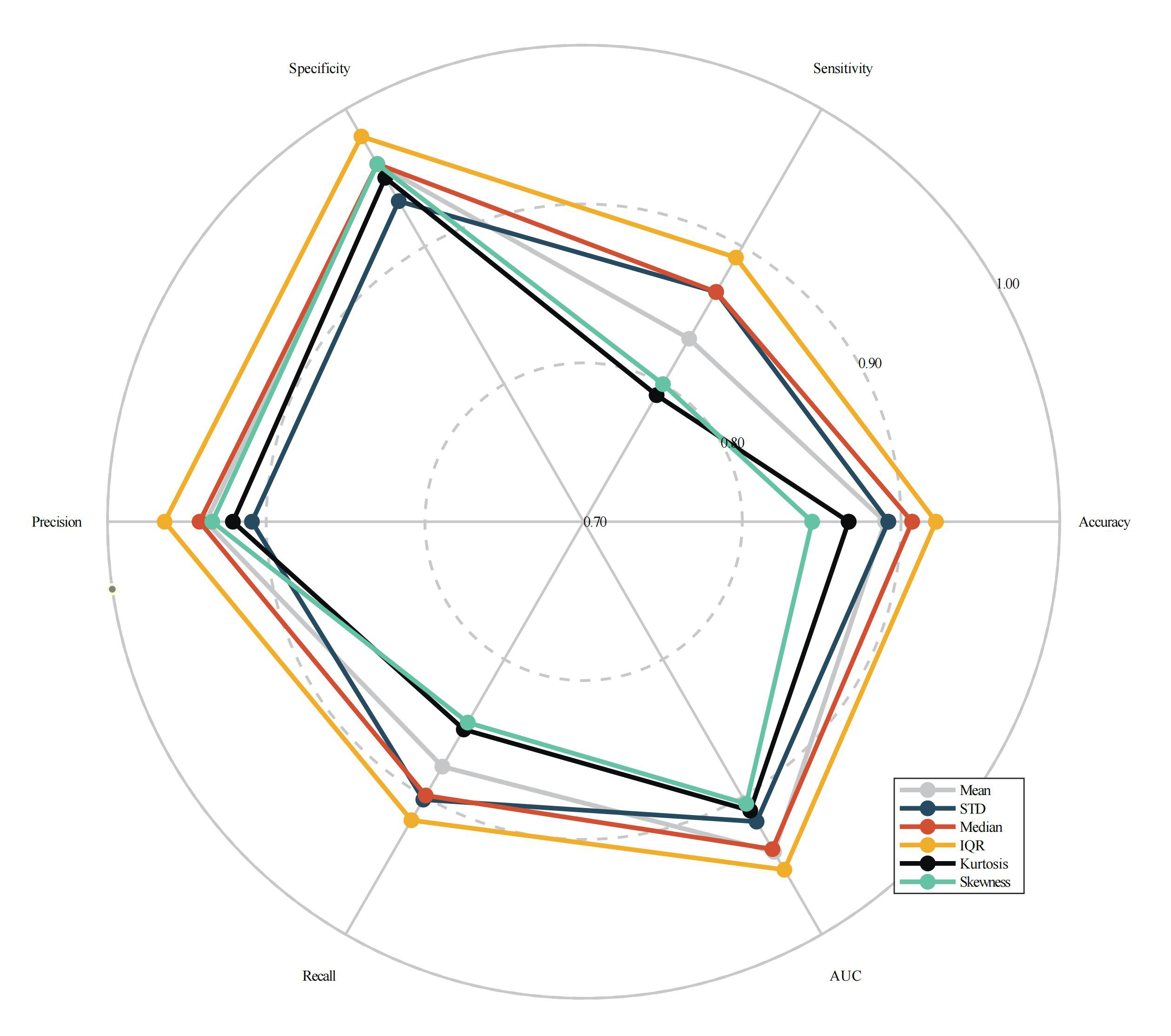 Fig. 6.
The radar plot of overall performance measures across all conditions for 6 dynamic graph-theory indicators.
The greatest results were obtained with a window width of 3 s and a movement step of 50%. Therefore, we investigated further by examining feature rankings and the distribution of particular features on scalp regions and frequency sub-bands. Table 6 presents the feature rankings and weights for 6 indicators of dynamic graph theory, in this condition. Features in the Beta and Alpha2 frequency sub-bands held the bulk of the top places, indicating that features in the high-frequency sub-bands had a greater contribution to the classification of individuals with ASD. In terms of mean, median, and IQR (all three indicators achieving 100% categorization), Beta-F3, Beta-F3, and Beta-Fp1 were the most significant features.
The proportion distribution of chosen characteristics across 6 dynamic graph-theory indicators in 5 frequency sub-bands is provided in Table 7. The results indicated that, with an unweighted proportion of 28%, and a weighted proportion of 40%, the features from the Beta sub-band had the dominant position. Similar to this, we investigated the distribution of particular traits on 5 regions of the scalp: parietal (P3, Pz, P4, P7, P8), temporal (T4, T5), occipital (O1, and O2), central (C3, Cz, C4), frontal (Fp1, Fp2, F7, F3, Fz, F4, F8), and parietal (P3, Pz, P4, P7, P8). It was evident that the frontal-area features that were chosen had the highest weighted proportion (46.153%) and unweighted proportion (36.364%). We also determined the relative relevance for the scalp region, taking into account that each region had a different number of channels. This was done by dividing the channel proportion (k/19, where k is the number of channels in a region). For instance, the frontal region’s unweighted relative relevance was 0.987, when 0.364 was divided by 7/19. Table 7 shows that, even after accounting for channel percentage, the weighted relative relevance of characteristics from the frontal region remained the highest (1.253).
| Scalp region | Proportion (%) | Relative importance | Weighed proportion (%) | Weighed relative importance | Frequency sub-band | Proportion (%) | Weighed proportion (%) |
| Parietal lobe | 26.263 | 0.998 | 24.659 | 0.937 | Alpha-1 | 14.141 | 10.124 |
| Frontal lobe | 36.364 | 0.987 | 46.153 | 1.253 | Alpha-2 | 33.333 | 27.298 |
| Temporal lobe | 11.111 | 1.056 | 6.9450 | 0.660 | Beta | 28.283 | 40.739 |
| Occipital lobe | 7.071 | 0.672 | 4.9120 | 0.467 | Delta | 6.061 | 4.899 |
| Central lobe | 19.192 | 1.215 | 17.331 | 1.097 | Theta | 18.182 | 16.939 |
The results showed that dynamic graph-theory indicators performed best when the window width and moving step were adjusted to 3 s and 50%, respectively. Some of them actually approached 100% accuracy.
The window-width setting in dynamic functional-connectivity analysis is still debatable and mostly dependent on researchers’ personal preferences. Previous research on dynamic functional connectivity demonstrated that although an excessively wide window width would obscure the information pertaining to dynamic transient shifting, an excessively small window width would raise the possibility of adding artifacts and lowering the frequency resolution [24]. Accordingly, it appears that a satisfactory compromise between frequency resolution and the capacity to capture variability was struck in the present study, since the 3-s window width yielded the maximum accuracy. The performance of the 3-s window-width dynamic graph-theory indicators marginally declined when the moving step was set to 100%, but it was still better than the 1-s and 5-s settings, which may provide additional support for choosing 3-s as the window width.
Another benefit in terms of preventing over-fitting was that we found that the number of selected features was lowest in the 3-s window-width and 50% moving-step conditions. One suggestion has been that when there are more features than subjects, over-fitting is more likely to happen [37]. The experimental results of Guyon et al. [36] demonstrated that the SVM algorithm benefits from feature reduction, even if SVM uses regularization approaches to partially avoid the over-fitting problem. Reducing the number of characteristics in the model enhances its interpretability while also reducing the possibility of overfitting. A model with fewer features is likewise simpler, requires less storage space, takes less time to compute, and possibly improves the model’s accuracy, because it contains fewer false positives. Features with higher interpretability and lower computation costs can offer a better understanding of the relationship between the input and output features, which is advantageous in situations in which resource efficiency is crucial [38, 39]. In summary, the 3-s window-width and 50% moving-step conditions allowed for the best classification performance with the fewest features needed. This finding should aid future research that uses dynamic functional-connectivity analysis regarding window-width and moving-step selection.
The IQR, an indicator that characterizes the dispersion and variance of the data distribution, had the highest accuracy among the 6 dynamic graph-theory indicators. This suggests that the value representing the variability of node strength had a significant ability to differentiate ASD patients from the control group. Only dFCA showed a significant difference in the study [40], suggesting that the functional-connectivity variability described by dFCA may offer distinct temporal information. The variability of functional connectivity reflects the instability of the information-transfer process within and between regions, and the flexibility of reconfiguration of one region with remaining regions [41].
Consistent with earlier research, the distribution analysis of a subset of features revealed a clear advantage of the frontal area. The frontal region was commonly identified as the aberrant portion using EEG or fMRI data in earlier research. The medial prefrontal cortex (mPFC) was identified as a hub of dysconnectivity in a study [42] that used lag-phase synchronization to construct functional connectivity on the cortical level, using a standardized low-resolution brain electromagnetic-tomography method. The mPFC plays an important role in the social cognition process. Similarly, several previous investigations identified aberrant functional connectivity in the default-mode network (DMN) in ASD patients [43, 44, 45]. Higher resting-state fronto-parietal-network (FPN)-DMN dynamics were linked to lower cognitive flexibility, according to one article [46]. According to Chen et al. [47], frontal-temporal connections in ASD connectivity demonstrated larger signal fluctuations. That suggested that increased variability of connection between these two regions could hinder the processing of social and cognitive information. The above results suggested that the there is an increased variability of functional connectivity between frontal region and other regions in ASD patients. However, reports of the opposite outcome also surfaced. Findings of Chen et al. [43] indicated that mPFC-insula connection variability was lower in ASD patients. Chen et al. [43] noted that the insula served as a core region of the salience network (SN), which suppresses executive function in the absence of external input, by strengthening its functional connectivity to the mPFC to preserve an internally focused state. However, in order to be alert for any modifications from the outside, the SN would sometimes alter the network configurations. Accordingly, a decreased variability in mPFC-insula connections could explain why ASD patients exhibit more internally directed cognition and respond less to the external world [43]. In summary, our findings indicated that the dynamic graph-theory indicators of node strength of the frontal region had the greatest significance in the diagnosis of ASD, suggesting that there are abnormal interactions between the frontal and other brain regions. These results may also reflect decreased and increased variability of the functional connectivity of the frontal region with other regions simultaneously, as well as an overall abnormality in the variability of topological characteristics in the frontal region.
We found that the Beta sub-band was the most significant of 5 frequency sub-bands (unweighted proportion 28.283%; weighted proportion 40.739%), indicating that high-frequency sub-bands may contain more information about the abnormality in ASD. The most significant features for mean, median, and IQR (these 3 indicators achieved 100% classification) were Beta-F3, Beta-F3, and Beta-Fp1. Beta-frequency coherence is believed to be related to cognitive and attentional functions [48, 49], and typically occurs in frontal and central region. Boersma et al. [50] observed that children with ASD have connection decrease in 51 ROI pairs, mainly in the Beta frequency. Additionally, they found that patients with ASD had significantly lower clustering coefficients and whole-brain average connection strengths in the Beta band than did controls. Research has indicated that people with ASD are less likely to be able to recruit Beta-band synchronization in large-scale networks, which could be a factor in the cognitive impairments that are common in ASD [51]. When the aforementioned information was combined with the findings of our feature-selection study, it became apparent that the aberrant variability of functional connectivity in the Beta sub-band may have the greatest impact on ASD diagnosis.
In a previous study [52], scientists classified ASD using the SVM algorithm, based on variables derived from brain functional connectivity across various frequency sub-bands obtained from fMRI. The best accuracy, according to the results, was 0.792. The Slow-4 (0.027–0.073 Hz) sub-band was found to include the majority of the discriminative features, and they found abnormal connections between the default mode network, the fronto-parietal network, and the cingulo-opercular network. Other research [53] classified children with ASD using the SVM model and used EEG to create a functional-connectivity network by partial correlation. They obtained the maximum accuracy at 0.800. When it came to dFCA, Price and his colleagues [27] extracted features from static and dynamic functional connectivity alternately, to match the multi-kernel support vector machine (MK-SVM) algorithm, and discovered that the dynamic feature could obtain a greater accuracy (0.900). Nevertheless, these studies only used the original functional connectivity as features to fit the model, and the ranking of feature importance was not involved. In order to differentiate ASD patients from normals, one study [54] used an ensemble classification model in conjunction with the SVM-RFE, and discovered that the posterior cingulate gyrus and precuneus had the highest ranking in terms of connection. Other researchers [55] used 5 global graph-theory indicators to attain an accuracy of 0.958 in their research using graph theory for the diagnosis of ASD. Another study [21] used a feature priority ranking by computing the node degree to fit the SVM model. The default mode network demonstrated a comparatively high network degree and discriminative capacity, and they were able to get 0.958 accuracy. In contrast to the previous research, ours has the advantage of combining indicators from local graph theory, dynamic functional connectivity, and ranking of future importance, all at once. This allowed us to make use of the dynamics information from dFCA and rank the selected features to identify the most significant ones, offering a fresh viewpoint on ASD diagnosis.
There are several limitations to our investigation. First, because a 19-channel EEG was used, source reconstruction could not be performed to find the EEG signals at the brain level. In order to improve this, we advise that future research employs EEG recording devices with greater spatial resolution in order to gather proof of convergence between fMRI and EEG. Second, the cross-sectional-data type affected the possibility of clarifying the mechanisms underlying ASD. We anticipate that future research will incorporate longitudinal follow-up EEG to compile data from the development track, in order to improve classification performance and to offer an alternative viewpoint for evaluating the course of the disorder. Third, there is a need for external validation and an increase in sample size. We intend to perform our study on a bigger external-validation dataset in the future.
Our research showed that dynamic local graph-theory indicators yielded the greatest classification performance and required fewer features in the optimal feature subset, when we used a 3-second window width and a 50% moving step. The outcomes of the feature-selection process demonstrated a distinct advantage for the frontal region and the Beta band. This suggested that the frontal-region dynamics underwent modifications in its functional-connectivity interactions with other regions, particularly in the Beta sub-band. These findings provide novel insights into exploration of biomarkers for the diagnosis of ASD.
Data related to the current study are available from the corresponding author on reasonable request.
JXZ and HL were responsible for conceptualization; HL was responsible for methodology; HL performed formal analysis and investigation; HL wrote the original draft; JXZ, SY, NXZ, LEH, YFG, AC and JPZ were responsible for review and editing; AC and JPZ provided resources. The algorithm concept and design of this paper were contributed by all authors. All authors also participated in the experimental evaluation. All authors contributed to editorial changes in the manuscript. All authors read and approved the final manuscript. All authors have participated sufficiently in the work and agreed to be accountable for all aspects of the work.
The study was conducted in accordance with the Declaration of Helsinki and approved by the Ethics Committee of the School of Public Health in Sun Yat-sen University (2021-No.081). Informed consent was obtained from the parents of all subjects involved in the study.
The authors would like to thank the participants of the Department of Pediatrics and the Department of Science and Education of Zhongshan Bo’ai Hospital (Zhongshan, China) for supporting the data collection of this study.
This research was funded by the Guangdong Basic and Applied Basic Research Foundation under Grand No. 2022A1515011237.
The authors declare no conflict of interest.
Publisher’s Note: IMR Press stays neutral with regard to jurisdictional claims in published maps and institutional affiliations.