
Amino acid nutrition studies often involve repeated measures data. An example is that the concentrations of plasma citrulline in steers are repeatedly measured from the same animals. The standard repeated measures ANOVA method does not detect significant time changes in the concentrations of plasma citrulline within 6 hours after steers consumed rumen-protected citrulline, while a graphical analysis indicates that there exists a time effect. Here we describe three mixed model analyses that capture the time effect in a statistically significant way, while accounting for the correlations of measurements over time from the same steers. First, we allow flexible variance-covariance structures on our model. Second, we use baseline measurements as a covariate in our model. Third, we use percent-change from baseline as a data normalization method. In our data analysis, all these three approaches can lead to meaningful statistical results that oral administration of rumen-protected citrulline enhances the concentrations of plasma citrulline over time in ruminants. This supports the notion that rumen-protected citrulline can bypass the rumen to effectively enter the blood circulation.
Repeated measures data often arise from nutrition research with animals (1-4). For example, in a study to evaluate the degradation of amino acids from the rumen of adult steers (5), the concentrations of citrulline in plasma are repeatedly measured from each animal at six different time points (Figure 1). The scientific hypothesis of this study is that oral administration of citrulline may enhance its plasma concentrations over time in adult steers. This seems quite obvious when studying the average trajectory of the concentrations of plasma citrulline at each time point (Figure 3); it increases at earlier times (between time t = 0 and time t = 1) and eventually decreases after time t = 4. Therefore, the main question is to assess whether time is an important factor in the mean changes of plasma citrulline concentrations using valid statistical methods.
 Figure 1.
The individual trajectories of the concentrations of citrulline in the plasma of all steers (n=6) over study time for the raw data. There is the high variability in citrulline concentrations among steers at the baseline as well as at the post-baseline time points.
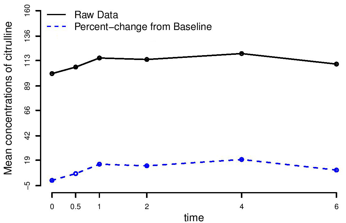 Figure 3.
The average trajectories of the mean concentrations of citrulline for the raw data and for the normalized data, whose patterns are similar. The average concentrations of citrulline tend to increase very rapidly up to time t =1 hour, slightly increase between times t = 1 hour and t = 4 hours and eventually decrease after time t = 4 hours.
One way to analyze this type of experimental data is to use a linear mixed effects model (6). With fixed time periods of measurement, this is also a repeated measures problem. This methodology can account for variability among and within the steers as well as the correlation of the measurements within the steers. In this framework, there are multiple options for analysis, and we explore three such options, along with sub-options dealing with the within-steer correlations.
Two crucial considerations drive the analysis of the data. One issue is that at the study baseline, there are very noticeable, large differences in the concentrations of plasma citrulline among the steers (Figure 1). If not accounted for, this unexplained variation greatly decreases the statistical power for detecting time effects. The other issue is how to capture the correlation of the repeated measured data within individual steers. Another potential issue is the possibility that the variance of the measurements may depend on time, often called heteroscedasticity.
The main objective of our paper is to introduce three sensible strategies based on a linear mixed effects model to generate valid statistical results. Our strategies capture the huge biological variations among all study subjects and account for the correlations between measurements within individual subjects. The first strategy uses a linear mixed effects model with a properly selected variance-covariance structure. This will help to account for the relationship between measurements, particularly from the same animals. The second strategy introduces baseline measurements as a covariate (7) in the model. This strategy enables us to decrease variability in random errors and, therefore, increases the probability of detecting the significant time effect on the mean responses in the post-baseline analysis. The last strategy uses percent-change from baseline as the response, where all measurements from the same experimental unit are divided by their baseline value for each unit (e.g., steer). Using percent-change from baseline is a sensible and objective way to remove variability among the steers, and increase statistical power of our analysis, while still having an easily understood structure. Finally, we will show that these three statistical approaches, when properly applied, detect significant changes in mean concentrations of plasma citrulline over time.
In general, mixed effects models (6) incorporate two effects: a fixed effect and a random effect. The fixed effect is the main parameter of interest, which affects changes in response variables across animals. In our steer data (5), the main interest is the change in mean concentrations of plasma citrulline for all steers at each time point t = 0.0, 0.5, 1.0, 2.0, 4.0, and 6.0. Thus, the fixed effects should be the time effect with six levels that affects those citrulline concentrations. For example, the intercept of the fixed effects will be the mean effect of the citrulline concentrations at time t =0. These time effects do not vary across the experimental units (e.g., steers).
The random effect is a parameter, which varies among experimental units. This random parameter helps to account for subject-specific effects on response variables. In our steer data (5), we consider a random intercept as a random effect because the random intercept is associated with the particular steers, which are randomly selected from whole population of the interest (6). This implies that the concentrations of plasma citrulline over time will be different among the steers because of subject-specific effects. Particularly, the baseline measurements in our steer data differ considerably among six steers, meaning that the variability of the baseline measurements is very large. This huge variability makes distinguishing statistically significant time trends more difficult.
In this paper, we consider a linear mixed effects model, where both the time effect and the random intercept are linearly associated with the response variables. Specifically, the mean concentrations of citrulline (response variable) are associated with the time effects having six levels (explanatory variables) at each time point t = 0.0, 0.5, 1.0, 2.0, 4.0, and 6.0 in what is called a cell-means form. The random intercept in our model helps to quantify the subject-specific effects on the mean concentrations of plasma citrulline among steers.
Our linear mixed effects model has two sources of random variables. One is the random baseline values (random intercept) for each steer, which captures the biological variation among steers at baseline and then subsequent time points. The other is the within-steer error among time points for all steers, which comes from random fluctuations of measurements within a steer.
To begin with, we can assume a random intercept model as the simplest mixed effects model. Under the random intercept model, both the random intercept and the within-steer error for all steers are assumed to be independent, normally distributed with mean zero and constant variance. However, the independence assumption for the within-steer error does not seem appropriate for our repeated measures steer data. The main reason is that any two response variables (e.g., the concentrations of plasma citrulline) taken on the same steer must be correlated with each other. Moreover, it is possible that the within-steer variability changes over time.
This simple random intercept model must be modified by addressing a correct variance-covariance structure for our repeated measures steer data (Figure 1), which have a complex pattern of variability and correlation across time. To end this, we will explore more complex within-steer covariance structures in the following section.
We consider the three objective statistical approaches that can help explain all sources of variability and correlations in our steer data. They can also improve the possibility of detecting the significant time effect in our study. To find the most powerful model to fit our steer data, we will describe a data-based strategy for exploring different possible variance and correlation possibilities.
Mixed effects models allow flexible variance-covariance structures to capture variability and correlation between response variables among time points for all animals. We consider the following five variance-covariance structures under our linear mixed model:
(1) Standard covariance structure
The standard covariance structure assumes that all responses have the same variance over time, and that the correlation in the repeated measures within a steer is also constant. This is the same as having random intercepts in the model.
(2) Unstructured covariance structure
The unstructured covariance structure allows unequal variances and unequal correlations between the outcome variables measured at different time points. This structure is useful when there are a large number of observations in the data set, but it is problematic and numerically unstable in problems such as ours when the number of animals is very small.
(3) Autoregressive with order 1
The autoregressive with order 1 (AR(1)) assumes equal variances and correlations that only depend on distance between two time points where response variables are measured. For the correlation parameter -1 ≤ ρ ≤ 1 for any two response variables, if the distance between two time points is m units, the correlation between those two responses is ρm. For example, two response variables from the same steer that are closer in time are more correlated than those variables that are farther apart (8). The AR(1) structure assumes equally spaced time points.
(4) Exponential covariance structure
The exponential covariance structure (6) generalizes the AR(1) structure to unequally spaced time points. All other assumptions are the same as ones for the AR(1) structure.
(5) Unequal variability over time
The aforementioned variance-covariance structures in (1), (3) and (4) can be extended to have unequal variances (on main diagonal) across time points. The variance function takes different values depending on the particular steer at all different times of measurements.
To choose a correct variance-covariance structure, it is important for us to understand the experimental design, treatment structures, and the meaning of the covariance structures. Current literature (6, 9-10) summarizes various variance-covariance structures. The goodness-of-fit criteria also can help us to choose a mixed effects model with a correct variance-covariance structure. For example, the Akaike information criterion (AIC) is an estimation algorithm that does not depend on user-choice. Among a set of models, the AIC chooses a model that loses the least information. The model with the lowest AIC is preferred.
The first way of handling baseline measurements is to use the baseline as a covariate in our linear mixed effects model. We fit this model with the baseline covariate to our steer data containing only measurements at time t = 0.5, 1.0, 2.0, 4.0, and 6.0 (i.e., post-baseline measurements). This strategy will exclude the large variability of the baseline measurements from the steer data. It can help to reduce both among and within-steers variations in the post-baseline analysis and, therefore, increase the probability of detecting the significant mean changes in response variables over post-baseline times.
The second method for handling baselines is the percent-change from baseline. The percent-change from baseline normalizes the repeated response variables for steer at time t, by computing
where is the baseline response measured at time t =0 for all steers
The normalized baselines are all zeros at time t = 0 and, then, naturally excluded in the analysis. The post-baseline normalized responses are used in the analysis at time t = 0.5, 1.0, 2.0, 4.0, and 6.0. Using the percent-change from baseline method allows us to remove the massive baseline variation and, thus, can lessen post-baseline variation among animals. The important condition for using this method is that, because of taking ratios, the baselines must not be too close to zero. For example, if the baseline is very small such as for one animal, the percent-change from baseline makes post-baseline normalized data very variable, which decreases statistical power of our analysis to capture the time effect. Thus, the normalizing data process not only reduces the existing high variability among animals at each time point, but also stabilizes the variability of within-animals error. It enables our statistical method to detect significant changes of mean response variables over time more easily, thus it is scientifically more justified rather than using the raw data. The graphical reasoning is given in Figure 2 and Figure 3, which shows the individual trajectories and the mean trajectory of the normalized values for the concentrations of plasma citrulline from six steers.
 Figure 2.
The individual trajectories of the concentrations of citrulline in the plasma of all steers (n=6) over study time for the normalized data using the percent-change from baseline method. After normalizing measurements, the baseline measurements become 0 for all steers and, thus, the high variability in the citrulline concentrations were reduced among steers at each time point.
After we applied our linear mixed effects model to the steer data (5), we conducted the analysis of variance test. For the repeated measures ANOVA test, we let .jbe the population mean concentration of plasma citrulline at the th level of the time factor, where and 6. We tested whether the mean concentrations of plasma citrulline .j are the same at different levels of the time factor, so that the null hypothesis is for all animals.
Using the R code (Section 8 of this paper), we applied our repeated measures ANOVA test to the steer data (5). Randomly chosen six steers were fed a diet, which was supplemented with 0.5 percent citrulline. We obtained blood from the jugular vein of each steer prior to feeding the treatment diet (t = 0). We also took blood samples repeatedly at time t = 0.5, 1.0, 2.0, 4.0, and 6.0 hours from each steer on day 15 (Figure 1) after all steers consumed the supplement.
Our objective in these analyses is to assess whether the mean concentrations of citrulline in the plasma of all steers are different at each level of the time factor t = 0.0, 0.5, 1.0, 2.0, 4.0, and 6.0. This can be done by assessing the fixed time effect at each level of the time factor and the random intercept (random effect), which captures existing biological variation on the mean concentrations of plasma citrulline among steers at each time point. When we use percent-change from baseline as a normalization procedure, we use the independent t-test to see if the rate of change in the concentrations of plasma citrulline is increasing at each time point.
We carried out three approaches in our analyses. First, we fit our linear mixed effects model with the exponential covariance structure by allowing unequal variances at all time points across all steers. For the post-baseline analysis, we handle the baselines by: 1) using the baseline as a covariate method, and 2) normalizing data by the percent-change from baseline method. Here, we also consider the same correlation structure used in the first method. Among other possible covariance structures, the AIC chose the linear mixed effects model with exponential covariance structure having unequal variances at all different time points across steers (our final linear mixed effects model for the analysis study). We compared the analyses results from our linear mixed effects models based on the three approaches to the result from the random intercept model, which assumes equal variance and constant correlations among all steers at all time points.
Our linear mixed effects model using the three strategies outlined above can capture the biological variations in the concentrations of plasma citrulline among all steers and the repeated measures ANOVA test shows that the mean concentrations of plasma citrulline change over time. The overall time factor is statistically significant with p-values of < 0.001 from the three approaches (Table 1). However, the traditional repeated measured ANOVA model based on the random intercept model failed to detect significant changes in the concentrations of plasma citrulline over time, with p-value 0.064 (Table 1). This is because the random intercept model cannot capture the important features of our steer data, which have varying correlations between response variables from the same steers over time and have different variances at all times across all steers.
| Procedure | Repeated Measures ANOVA | |
| Covariance | P-value | |
| Standard Method | Random Intercept | 0.064 |
| Var-Cov Structure | Hetero Exponential | <0.001 |
| Baseline Covariate | Hetero Exponential | <0.001 |
| Percent-Change from Baseline | Hetero Exponential | <0.001 |
| 1 The data indicate the probability values from our analyses of the concentrations of citrulline in the plasma of steers (n=6) using the repeated measures ANOVA across the factor Time. There are four analyses: (a) the standard method that simply has a random intercept, forcing the equal variances and equal correlation across time; (b) the modification of (a) that allows different variance-covariance structures; (c) making the baseline concentration as a covariate, and (d) normalizing the data using percent-change from baseline as the response. For (b)-(d), we allow our linear mixed effects models to have different variance-covariance structures, and the goodness-of-fit criterion (AIC) chose each model with the exponential covariance structure having heteroscedastic (different) variances at the different time points. Method (a) shows no statistically significant effect largely because the variances change with time as do the correlations in our data. | ||
With the normalized data using the percent-change from baseline method, we found that mean concentrations of plasma citrulline increase during the initial time points after the oral administration of citrulline. Our analysis result shows that the effects of the fixed time factor at levels t = 1, 2 and 4 are positive with the corresponding small p-values, respectively, in Table 2.
| Time | Percent-change from baseline/ Average of concentrations of citrulline (p-value) |
| 0.5 | 6.389 (0.184) |
| 1 | 15.245 (0.037) |
| 2 | 13.733 (0.005) |
| 4 | 19.691 (0.001) |
| 6 | 9.720 (0.257) |
| 1The data indicate the fixed time effects on the concentrations of citrulline in the plasma of all steers (n=6) with the corresponding probability values (p-values) at each time point t = 0.5, 1, 2, 4, 6. This analysis proceeded under the percent-change from baseline method. Based on the p-values, we showed that the mean concentration of citrulline is statistically significantly increasing at time t = 1, 2, 4. | |
Our results, which are properly analyzed by the three objective statistical approaches, have very important nutritional importance. Amino acids are extensively degraded in the ruminant rumen and that they may not have nutritional values unless encapsulated through time-consuming and expensive technologies (11). This is true for arginine and glutamine, because oral administration of these two amino acids do not increase their concentrations in the plasma of adult ruminants (5). However, rumen-protected citrulline can escape the rumen of adult steers to enter the blood circulation, thereby increasing citrulline concentrations in their plasma. This indicates that ruminal microbes do not degrade the encapsulated citrulline. Our finding has important implications for human health. For example, it is known that arginine, the physiological product of citrulline via argininosuccinate synthase and lyase in virtually all cell types (12), can inhibit the early stage of tumorigenesis in the colon (13) that harbors a large amount of microbes. Because the conversion of citrulline into arginine consumes ammonia (a toxic molecule at high concentrations (14, 15)) and because arginine can be actively degraded by intestinal microbes (16), the use of oral citrulline rather than arginine may increase the bioavailability of arginine to colonocytes, thereby reducing risk for colon cancer.
Our analysis procedures using three statistical strategies sensitively captured the changes in the concentrations of plasma citrulline over time after steers received oral administration of citrulline. We considered a cell-means form of linear mixed effects model and correctly accounted for the correlations between measurements. In all methods, constructing a correct variance-covariance structure is important since it can correctly explain the important characteristics of the given data and affects to the analyses results. Adjusting for the variability of the baseline measurements is important in this steer data as there is high variability among animals at initial time point. Handling baseline measurements techniques using the baseline as a covariate and the percent-change from baseline methods will reduce those high variability among animals at the initial time and thereafter. Thus, the random errors in steer data become stable and it can improve statistical power of analysis to detect the significant overall time effect on the mean changes of the plasma citrulline concentrations. Particularly, we can use the percent-change from baseline method as a data normalization technique as long as the baseline measurements are very far away from zero. The presented statistical procedures are not limited to the analysis of data for plasma amino acids. These procedures can help nutritionists to think independently when they hope to analyze their experimental data and answer their own scientific questions.
The following R code has been employed to analyze our repeated measures steer data using three statistical approaches: the various variance-covariance structure, the use of baseline as a covariate, and normalization of data as percent-change from baseline methods. To run this function, we have installed the “nlme” package in the R program. Data must be in the long format with animal id, group, time, and outcomes (e.g., amino acids) as columns in an excel file. The data file must be saved as a .csv file. This R code generates the data in Table 1 and Table 2, as well as Figures Figure 1, Figure 2, and Figure 3.
## Input parameters:
## num.aa: the number of amino acid
## n: the number of animals
## time.points: the number of time points that are considered in the analysis
## interv.length: interval length for the y axis in the graph
## num.method: how many number of methods you will use in the analysis
anova.test<-function(num.aa=1, n=6, time.points=6, interv.length=7, num.method=4, file="cit_data.csv"){
## read the steer data
steer<- read.csv(file=file)
## true name of outcomes to return plots with true amino names
true.AA<-names(steer)(4)
## assign column names
colnames(steer)<-c("Steer", "Group", "Time", "AA")
## dummy variables for steers and time
## steers are six distinct steers; time factor has 6 levels (t=0, 0.5, 1, 2, 4, 6), where 0 is the reference level
tag<-factor(steer$Steer)
time<-factor(steer$Time)
## preparation of steer data in the data.frame format for the analysis
## tag is the categorical variable with 6 distinct steers; time is the categorical variables with 6 levels
steer<-cbind(steer, tag, time)
steer<-do.call("data.frame", steer)
## obtain specific name for amino acids to be analysis
amino.names<-names(steer)((3+1))
##############################################
# Method 1: Modeling variance-covariance structure ##
##############################################
###{{
## Initialization for the array of output
lme.model.selec<-array(0,dim=c(3, 3, num.aa), dimnames=list( c("Model0",
"Model1", "Model2"), c("Model", "df", "AIC"), "Method1" ))
lme.results<-array(0,dim=c(2, 1, num.aa), dimnames=list( c("intercept", "Time"),
c("P-value"), amino.names ))
lme.cov.results<-array(0,dim=c(2, 1, num.aa), dimnames=list( c("intercept", "Time"),
c("P-value"), amino.names ))
## analysis for method 1
for (i in 1:num.aa){
## mixed model (cell-means form) with standard var-cov structure
model0<-lme(AA~time, data=steer, random=~1|tag)
lme.anova0<-anova(model0)
## summary for anova results -with constant
lme.anova.summary0<-lme.anova0( , "p-value")
lme.results( , , i)<-round(lme.anova.summary0, 3)
## various variance-covariance structure:
## 1) Standard structure
## 2) Exponential (generalized AR(1)): correlation decreases depending on distance between two
## observations from the same steer. Two observations are closer in time have higher correlation than
## those are further.
## 3) Exponential with unequal variances:
## varIdent: variance function structure allows different variances for each level of a factor
## exponential model
model1<-lme(AA~time, random=~1|tag,
correlation=corExp(form = ~1|tag, nugget=TRUE), data=steer)
## exponential model with unequal variances
model2<-lme(AA~time, random=~1|tag, weights=varIdent(form=~1|tag),
correlation=corExp(form = ~1|tag, nugget=TRUE), data=steer)
## Model selection: Standard cov vs. Exponential vs. Exponential with unequal variances
## choose a model with smallest AIC
ano.test1<-anova(model0, model1, model2)
lme.model.selec<-cbind(ano.test1(, "Model"),ano.test1( , "df"), ano.test1( , "AIC"))
colnames(lme.model.selec)<-c("Model", "df", "AIC")
rownames(lme.model.selec)<-c("standard", "Exp", "Exp.hetero")
## Choose the lowest AIC
lme.anova1<-anova(model2)
## summary for anova results
lme.anova.summary1<-lme.anova1( , "p-value")
lme.cov.results( , , i)<-round(lme.anova.summary1, 3)
}
###}}
###################################
# Method 2: Using baseline as a covariate ##
###################################
## unique steer with tag number
uniq.steer<-unique(steer$tag)
###{{
## Initialization for data structure
trim.steer.base.cov<-vector("list", n)
##Create subdata by changing baseline as a covariate
for (id in 1:length(uniq.steer)){
# Initialization to have baseline as covariate
subdata<-steer(steer$Steer==uniq.steer(id), )
base.amino<-matrix(100, nrow=(time.points-1), ncol=num.aa)
## get data structure for response variables at time t=0.5, 1, 2, 4, 6 and baseline covariates
for (j in 1:num.aa){
base.amino( , j)<-rep(subdata( , amino.names(j))(subdata$time==0), (time.points-1))
}
trim.subdata<-subdata(-1, )
colnames(base.amino)<-paste("base.", amino.names, sep="")
## subdata without baselines
trim.subdata.base.amino<-cbind(trim.subdata, base.amino)
trim.steer.base.cov((id))<-trim.subdata.base.amino
}
## change data structure to data.frame from list type
trim.steer<-do.call("rbind.data.frame", trim.steer.base.cov)
## Initialization for analysis
lme.base.model.selec<-array(0,dim=c(3, 3, num.aa), dimnames=list( c("Model0", "Model1",
"Model2"), c("Model", "df", "AIC"), "Method2" ))
lme.base.cov.results<-array(0,dim=c(3, 1, num.aa), dimnames=list( c("intercept", "baseline",
"time"), c("p-value"), amino.names))
## Fit model with baseline covariate with specific var-covariance structure
for (i in 1:num.aa){
#with standard structure
model3<-lme(AA~1+base.AA+time, random=~1|tag, data=trim.steer)
#with exponential structure
model4<-lme(AA~1+base.AA+time, random=~1|tag,
correlation=corExp(form = ~1|tag, nugget=TRUE), data=trim.steer)
#with exponential structure with unequal variances
model5<-lme(AA~1+base.AA+time, random=~1|tag, weights=varIdent(form=~1|tag),
correlation=corExp(form = ~1|tag, nugget=TRUE), data=trim.steer)
## Model selection: Standard cov vs. Exponential vs. Exponential with unequal variances
## choose a model with smallest AIC
ano.test2<-anova(model3, model4, model5)
lme.base.model.selec<-cbind(ano.test2( , "Model"),ano.test2( , "df"), ano.test2( , "AIC"))
## give column and row names
colnames(lme.base.model.selec)<-c("Model", "df", "AIC")
rownames(lme.base.model.selec)<-c("standard", "Exp", "Exp.hetero")
## Choose the lowest AIC
lme.anova2<-anova(model5)
## Anova results
lme.anova.summary2<-lme.anova2( , "p-value")
lme.base.cov.results( , , i)<-round(lme.anova.summary2, 3)
}
###}}
####################################
# Method 3: Normalizing data as percent-change from baseline ##
####################################
##{{
## Initialization for Normalized data
no.base.steer.list<-vector("list", n)
uniq.steer.list<-vector("list", n)
## analysis for method 3
for (id in 1:length(uniq.steer)){
## obtain subdata for each steer
subdata<-steer(steer$Steer==uniq.steer(id), )
## Initialize matrix for normalized amino acids data at each time point
normamino<-matrix(100, nrow=time.points, ncol=num.aa, dimnames=list(c("time0",
"time0.5", "time1" , "time2" , "time4" , "time6"), amino.names))
for (j in 1:num.aa){
## %-change from baselines: divide all response variables by baselines
baseamino<-subdata( , "AA")(subdata$time==0)
normamino(, j)<-{{(subdata( ,"AA")/baseamino)}*100}-100
subdata(, c(paste("norm.", amino.names, sep="")))<-normamino(, j)
}
## normalized baselines are all 0; subdata has only data at time 0.5, 1, 2, 4, 6
uniq.steer.list((id))<-subdata
## normalized baselines are excluded in the analysis
no.base.subdata<-subdata(-1, )
no.base.steer.list((id))<-no.base.subdata
}
## normalized data set by using percentage-change from baseline
nobase.trans.steer<-do.call("rbind.data.frame", no.base.steer.list)
## exclude the original scaled response varibles
trans.steer<-nobase.trans.steer(,-((3+1):(3+num.aa)))
## obtain specific name for normalized amino acids to be analysis
norm.amino.names<-names(trans.steer)(6)
## initialization for analysis results
lme.percent.model.selec<-array(0,dim=c(3, 3, num.aa), dimnames=list( c("Model0",
"Model1", "Model2"), c("Model", "df", "AIC"), "Method3" ))
lme.percent.results<-array(0,dim=c(1, 1, num.aa), dimnames=list( c("Time"),
c("P-value"), norm.amino.names))
## fit mixed effects model to percentage-based from baselines
for (i in 1:num.aa){
##with standard structure
model6<-lme(norm.AA~-1+time, data=trans.steer, random= ~1|tag )
##with exponential structure
model7<-lme(norm.AA~-1+time, data=trans.steer, random= ~1|tag,
correlation=corExp(form = ~1|tag, nugget=TRUE))
##with exponential structure with unequal variances
model8<-lme(norm.AA~-1+time, data=trans.steer, random= ~1|tag,
weights=varIdent(form=~1|tag), correlation=corExp(form = ~1|tag, nugget=TRUE))
## Model selection: Standard cov vs. Exponential vs. Exponential with unequal variances
## choose a model with smallest AIC
ano.test3<-anova(model6, model7, model8)
lme.percent.model.selec<-cbind(ano.test3(, "Model"),ano.test3(, "df"), ano.test3(, "AIC"))
## column and row names
colnames(lme.percent.model.selec)<-c("Model", "df", "AIC")
rownames(lme.percent.model.selec)<-c("standard", "Exp", "Exp.hetero")
## Choose the lowest AIC
lme.anova3<-anova(model8)
## analysis results
lme.anova.summary3<- lme.anova3(,"p-value")
lme.percent.results( , , i)<-round(lme.anova.summary3, 3)
}
###}}
###{{ Combine all analysis results using linear mixed effects model for Table 1
combine.results<-array(0,dim=c(num.method, 1, 1), dimnames=list( c("lme.stand", "lme.cov",
"lme.base.covr", "lme.precent"), c("p-value"),"Time"))
## obtain results only for the time factor
## 1) with standard covariance structure
combine.results("lme.stand", ,"Time")<-lme.results(2, , "AA")
## 2) with heterogeneous variances and Exponential covariance structure
combine.results("lme.cov", ,"Time")<-lme.cov.results(2, , "AA")
## 3) with baselines covariates
combine.results("lme.base.covr", , "Time")<-lme.base.cov.results(3, , "AA")
## 4) with normalized data based on percent-change from the baseline
combine.results("lme.precent", ,"Time")<-lme.percent.results(1, , "norm.AA")
zero.pval<-which(combine.results( ,"p-value", "Time")==0)
combine.results( ,"p-value", "Time")(c(zero.pval))<-format.pval(combine.results( , "p-value",
"Time")(c(zero.pval)), eps=.001, ditis=2)
## return results without quotation mark on p-value
print(combine.results, quote=FALSE)
###}}
###{{ do independent t-test if the rate of concentrations of citrulline at each time point is increasing
## Initialization to have data summary: average and standard errors for each steer
percent.avr.at.times<-array(0,dim=c(2, 5, num.aa), dimnames=list( c( "avr", "sterr"),
c( "time0.5", "time1", "time2","time4", "time6"), norm.amino.names ))
## Initialization to have normalized data for each steer
percent.steer.at.times<-array(0,dim=c(6, 5, num.aa), dimnames=list( c( "steer1", "steer2",
"steer3", "steer4", "steer5", "steer6"), c( "time0.5", "time1", "time2","time4", "time6"), norm.amino.names))
## produce summary statistics including averages and standard errors for each steer
for (i in 1:num.aa){
aa<-i+5
## summary statistics at time 0.5
halfh.ind<-which(trans.steer$time==0.5); steer.at.halfh<-trans.steer( , aa)(halfh.ind)
avr.at.halfh<-mean( steer.at.halfh); str.at.halfh<-sd(steer.at.halfh)/sqrt(n)
## summary statistics at time 1
oneh.ind<-which(trans.steer$time==1); steer.at.oneh<-trans.steer( , aa)(oneh.ind)
avr.at.oneh<-mean(steer.at.oneh); str.at.oneh<-sd(steer.at.oneh)/sqrt(n)
## summary statistics at time 2
twoh.ind<-which(trans.steer$time==2); steer.at.twoh<-trans.steer( , aa)(twoh.ind)
avr.at.twoh<-mean(steer.at.twoh); str.at.twoh<-sd(steer.at.twoh)/sqrt(n)
## summary statistics at time 4
fourh.ind<-which(trans.steer$time==4); steer.at.fourh<-trans.steer( , aa)(fourh.ind)
avr.at.fourth<-mean(steer.at.fourh); str.at.fourth<-sd(steer.at.fourh)/sqrt(n)
## summary statistics at time 6
sixh.ind<-which(trans.steer$time==6); steer.at.sixh<-trans.steer( , aa)(sixh.ind)
avr.at.sixth<-mean(steer.at.sixh); str.at.sixth<-sd(steer.at.sixh)/sqrt(n)
### average of outcomes at each time points ###
avr<-cbind(avr.at.halfh, avr.at.oneh, avr.at.twoh, avr.at.fourth, avr.at.sixth)
### standard errors of outcomes at each time points ###
se<-cbind(str.at.halfh, str.at.oneh, str.at.twoh, str.at.fourth, str.at.sixth)
stat.summary<-round(rbind(avr, se), 4)
percent.avr.at.times( , , i)<-stat.summary
percent.steer.at.times( , , i)<-cbind(steer.at.halfh, steer.at.oneh, steer.at.twoh,
steer.at.fourh,steer.at.sixh)
}
##Initialization for independent t-test results
summary.ttest<-array(0,dim=c(5, 4, num.aa), dimnames=list( c( "time0.5", "time1", "time2",
"time4", "time6"), c( "outcome.avr", "T-value", "num.para","p.value"),
true.AA))
#################################################################
## independent t-test if slope of each level of time factor is increasing or not ##
## Test if ##
## H_0: mu_{t}=0 at each time point t ##
## H_1: mu_{t}>0 ##
#################################################################
for (i in 1:num.aa){
for (t in 1:(time.points-1)){
test.time.eff<-t.test(percent.steer.at.times(,t,i), mu=0, var.equal=FALSE,
alternative="two.sided", conf.level=0.95)
summary.ttest(t, , i)<-as.numeric(cbind(test.time.eff$estimate, test.time.eff$statistic,
test.time.eff$parameter, test.time.eff$p.value))
}
}
summary.ttest<-round(summary.ttest, 3)
###}}
###{{ Produce Figure 1. Individual trajectories by original scaled data
for (aa in 1:num.aa){
substeer<-steer
## sort tag numbers for distinct steers
steer.tag<-unique(substeer$Steer)
## choose unique steer
one.uniq.steer<-which(substeer$Steer==steer.tag(1))
one.uniq.steer.data<-substeer(one.uniq.steer,)
## obtain amino acids name : "CIT"
min.amino<-min(substeer( , "AA"))
max.amino<-max(substeer( , "AA"))
ylim<-round(c(min.amino-5, max.amino+25), 0)
## colors
cols<-c("black", "blue", "red", "seagreen", "purple", "orange")
## plot names for saving
file0<-paste("", true.AA, sep="")
origin.graph<-paste0(file0, "_raw_data", ".pdf")
pdf(file=origin.graph, width=8, heigh=6)
## obtain names of amino acids
yvalues<-one.uniq.steer.data( , "AA")
ylab.name<-paste("concentrations of ", true.AA,sep="")
## do plot
plot(one.uniq.steer.data$Time, yvalues,
ylim=ylim, type="o", ylab=ylab.name, xlab="time",
col=cols(1), cex.lab=1.5, lwd=2.5, axes=F)
for (id in 2:n){
uniq.steer<-which(substeer$Steer==steer.tag(id))
uniq.steer.data<-substeer(uniq.steer,)
lines(uniq.steer.data$Time, uniq.steer.data(,"AA"), type="o", lty=id, col=cols(id),
lwd=2.5)
}
## x-axis and y-axis frame for Figure 1
axis(1,at=c(one.uniq.steer.data$Time),labels=c(one.uniq.steer.data$Time), lwd=2.5)
interval<-(ylim(2)-ylim(1))/interv.length
ylabs<-round(seq(ylim(1),ylim(2), by=interval),0)
axis(2,at=c(ylabs),labels=c(ylabs), lwd=2.5)
## legend
legend(0,max(ylabs),paste("Steer ", steer.tag, sep="")(1:3), col=cols(1:3),
lty=c(1:3), bty="n", cex=1.3, lwd=2)
legend(2,max(ylabs),paste("Steer ", steer.tag, sep="")(4:n), col=cols(4:n),
lty=c(4:n), bty="n", cex=1.3, lwd=2)
dev.off()
}
###end Figure 1}}
###{{ Produce Figure 2. Individiual trajectories by normalized data using percentage-changes from baselines
## call normalized steer data
full.trans.steer<-do.call("rbind.data.frame", uniq.steer.list)
for (aa in 1:num.aa){
aa<-1; j<-3+aa
## remmove original scaled Citrulline concentraions
## with dummy variables for tag and time
trans.substeer<- full.trans.steer(,-((3+num.aa):(5+num.aa)))
### sort tag numbers for distinct steers ###
steer.tag<-unique(trans.substeer$Steer)
### choose unique steer ###
one.uniq.steer<-which( trans.substeer$Steer==steer.tag(1))
one.uniq.steer.data<- trans.substeer(one.uniq.steer,)
### obtain amino acids name ###
amino.name<-as.character(names(one.uniq.steer.data)(4))
min.amino<-min(trans.substeer(,amino.name))
max.amino<-max(trans.substeer(,amino.name))
ylim<-round(c(min.amino-5, max.amino+40), 0)
### plot name for Figure file and create Figure file using pdf format
file1<-paste("", true.AA, sep=""); percent.graph<-paste0(file1,"_percent_change",".pdf")
pdf(file=percent.graph, width=8, heigh=6)
## obtain names of amino acids
norm.yvalues<-one.uniq.steer.data(,"norm.AA")
norm.ylab.name<-paste("concentrations of norm.", true.AA,sep="")
## do plot
plot(one.uniq.steer.data$Time, norm.yvalues, ylim=ylim, type="o",
ylab=norm.ylab.name, xlab="time", col=cols(1), cex.lab=1.5, lwd=2.5, axes=F)
for (id in 2:n){
uniq.steer<-which(trans.substeer$Steer==steer.tag(id))
uniq.steer.data<-trans.substeer(uniq.steer, )
lines(uniq.steer.data$Time, uniq.steer.data( , "norm.AA"), type="o", lty=id,
col=cols(id), lwd=2.5)
}
## grid for x-axis and y-axis
axis(1,at=c(one.uniq.steer.data$Time),labels=c(one.uniq.steer.data$Time), lwd=2.5)
interval<-(ylim(2)-ylim(1))/interv.length
ylabs<-round(seq(ylim(1),ylim(2), by=interval),0)
axis(2,at=c(ylabs),labels=c(ylabs), lwd=2.5)
## legend
legend(0,max(ylabs),paste("Steer ", steer.tag, sep="")(1:3), col=cols(1:3),
lty=c(1:3), bty="n", cex=1.3, lwd=2)
legend(2,max(ylabs),paste("Steer ", steer.tag, sep="")(4:n), col=cols(4:n),
lty=c(4:n), bty="n", cex=1.3, lwd=2)
dev.off()
}
### end of Figure 2}}
###{{ Produce Figure 3
## Initialization to have data summary: average and standard errors for each
origial.scaled.summarystat<-array(0,dim=c(2, 6, num.aa), dimnames=list( c( "avr", "sterr"),
c("time0", "time0.5", "time1", "time2","time4", "time6"), paste("orig.scaled.", true.AA, sep="")))
##For original scaled data , obtain summary statistics, mean and standard errors
for (i in 1:num.aa){
aa<-i+3;
## summary stat at time 0
init.ind<-which(steer$Time==0)
avr.at.zeroh<-mean(steer( , aa)(init.ind)); sd.at.zeroh<-sd(steer( , aa)(init.ind))/sqrt(n)
## summary stat at time 0.5
halfh.ind<-which(steer$Time==0.5)
avr.at.halfh<-mean(steer( , aa)(halfh.ind)); sd.at.halfh<-sd(steer( , aa)(halfh.ind))/sqrt(n)
## summary stat at time 1
oneh.ind<-which(steer$Time==1)
avr.at.oneh<-mean(steer( , aa)(oneh.ind)); sd.at.oneh<-sd(steer( , aa)(oneh.ind))/sqrt(n)
## summary stat at time 2
twoh.ind<-which(steer$Time==2)
avr.at.twoh<-mean(steer( , aa)(twoh.ind)); sd.at.twoh<-sd(steer( , aa)(twoh.ind))/sqrt(n)
## summary stat at time 4
fourh.ind<-which(steer$Time==4)
avr.at.fourth<-mean(steer( , aa)(fourh.ind)); sd.at.fourth<-sd(steer( , aa)(fourh.ind))/sqrt(n)
## summary stat at time 6
six.ind<-which(steer$Time==6)
avr.at.sixth<-mean(steer( , aa)(six.ind)); sd.at.sixth<-sd(steer( , aa)(six.ind))/sqrt(n)
## combine summary statistics at each time point
avr<-cbind(avr.at.zeroh, avr.at.halfh, avr.at.oneh, avr.at.twoh, avr.at.fourth, avr.at.sixth)
se<-cbind(sd.at.zeroh, sd.at.halfh, sd.at.oneh, sd.at.twoh, sd.at.fourth, sd.at.sixth)
stat.summary<-round(rbind(avr, se), 2)
origial.scaled.summarystat( , ,i)<-stat.summary
}
###{{ Figure 3 for the average trend for the concentrations of citrulline
## obtain name for Figure file in pdf format
file2<-paste("", true.AA, sep=""); avr.graph<-paste0(file2,"_mean_concentrations",".pdf")
pdf(file=avr.graph, width=8, heigh=6)
##obtain x and y values
time.vec<-c(unique(steer$Time))
avr.raw.yvalues<-origial.scaled.summarystat(,,1)("avr", )
## add 0 at time0 for the percentage-changes from baselines
avr.norm.yvalues<-c(0, percent.avr.at.times(,,1)("avr", ))
## range of y values and name of y axis
ylim<-c(-5, 160)
ylab.name<-paste("mean concentrations of ", true.AA,sep="")
## do plot
## raw data
plot(time.vec, avr.raw.yvalues, ylim=ylim, type="o", ylab=ylab.name, xlab="time",
col=cols(1), cex.lab=1.5, lwd=2.5, lty=1, axes=F)
## normalized data
lines(time.vec, avr.norm.yvalues, type="o", col=cols(2), cex.lab=1.5, lwd=2.5, lty=2)
## legend
legend(0,160, c("Raw Data", "%-change from Baseline"), col=cols(1:2),
lty=c(1, 2), bty="n", cex=1.3, lwd=2)
## grid for x and y axis
axis(1,at=c(time.vec),labels=c(time.vec), lwd=2.5)
interval<-(ylim(2)-ylim(1))/interv.length
ylabs<-round(seq(ylim(1),ylim(2), by=interval),0)
axis(2,at=c(ylabs),labels=c(ylabs), lwd=2.5)
dev.off()
### end of Figure 3}}
## returns list of results: Tables 1, 2 and Figures Figure 1,Figure 2 and Figure 3 in your directory
return(list(summary.ttest=summary.ttest ))
}## end of analysis
This research was supported by funds from Texas A&M AgriLife Research and the Texas A&M University’s Department of Animal Science Mini-Grant program (Guoyao Wu). Unkyung Lee was supported by a training grant from the National Cancer Institute (T32-CA00301). Tanya Garcia was supported by a grant from the National Institute of Neurological Disorders and Stroke (K01-NS099343). Raymond Carroll was supported by a grant from the National Cancer Institute (U01-CA057030).
Abbreviations: AIC: Akaike information criterion; ANOVA: Analysis of variance